from xkcd.com

image source IKEA

Dealing with tables

Before we look at `join`s

`bind_rows()` and `bind_cols()`

These are like sticky-taping a table together

Make sure the rows/columns match!

image source commons.wikimedia.org by Jarekt

Joining data tables

A better term would be ‘zipping’

Various types of `join`

Most commonly we want

`inner_join`, or

`left_join`

`inner` retains only rows that find a match

`left` retains all left table rows whether they match or not

Specifying the join


            # table_to_join is the table we want to join
            # the by parameter specifies which column(s)
            # to base the join on
            result <- input %>%
              inner_join(table_to_join, by = ...)

For example


            welly_pop <- welly %>%
              inner_join(pop_table, by = "Meshblock")

Variable name matching

The function will match on any shared variable names

If the thing you want to match on has different names in the two tables, then do something like this:


            welly_pop <- welly %>%
              inner_join(pop_table, by = c("Meshblock" = "MB2013"))

Care is required

Especially concerning the types of join variables

If names and (especially) types don’t match, use mutate to make them!


            # If the types don't match, then best
            # to make them match before joining
            welly <- welly %>%
              mutate(MB = as.character(Meshblock))
            pop <- pop %>%
              mutate(MB = as.character(MBnumber))

            # I have made matching variables of the
            # name and type, so now I don't need to
            # specify, it will find the match:
            welly_pop <- welly %>%
              left_join(pop)

Checking variable types

Use as_tibble


            > as_tibble(welly)
            # A tibble: 5,196 x 39
               Meshblock MeshblockN AreaUnitCo AreaUnitNa UrbanAreaC UrbanAreaT UrbanAreaN
               <fct>     <fct>      <fct>      <fct>      <fct>      <fct>      <fct>
             1 MB 18850… 1885000    564022     Otaki For… 502        Rural (In… Rural (In…
             2 MB 19038… 1903802    564601     Moonshine… 502        Rural (In… Rural (In…
             3 MB 19247… 1924700    569202     Alicetown  018        Main Urba… Lower Hut…
             4 MB 19526… 1952600    568502     Epuni East 018        Main Urba… Lower Hut…

Many possible types, but mostly you see

`<int>`, `<dbl>`, `<chr>` or `<fct>`

image source flickr.com/jeffsand by Jeff Sanquist
under a CC-BY-2.0 license

Name/type mismatches are common problems

Look out for

leading 0s
leading or trailing spaces
capitalisation, macrons, stray punctuation...

Fix issues using functions in the `stringr` package

Usually the `character` type is reliable

The `factor` type can do unexpected things

# Spatial joins ## Same idea, but the ‘zipper’ is a *spatial predicate* ## That is, some spatial relation between two datasets must hold ## The function this time is `st_join` from the `sf` package

# Notes ## A spatial join is a `left_join` by default, `left=FALSE` will make it an `inner_join` ## If more than one element in join dataset matches, you get duplicate entries in the joined dataset ## You have to consider what to do if you want to recombine them

‘Dissolving’ geometries

Accomplished by a non-spatial `dplyr` operation followed by a `summarise`


            states <- l48 %>%
                group_by(state) %>%
                summarise()

            states <- l48 %>%
                group_by(state) %>%
                summarise(across(where(is.integer), sum))

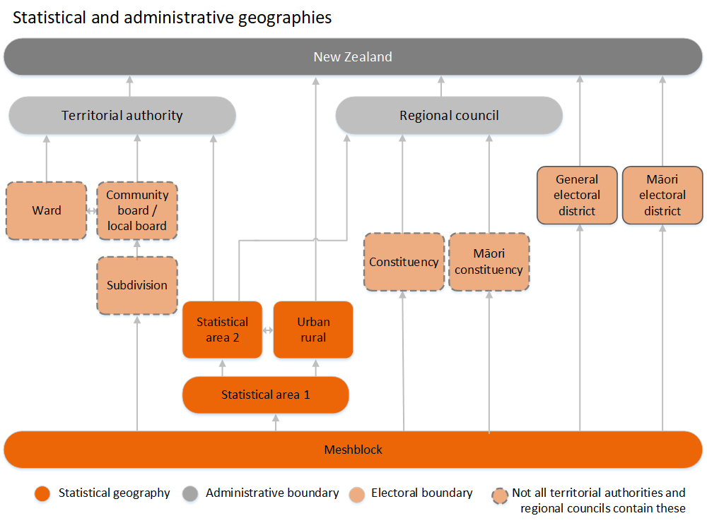
See this page at Statistics NZ for more details

New Zealand census geography

Meshblocks are the base level

Everything else is made from these, via concordance tables

The Statistics New Zealand geographic boundary viewer

# Summary ## Tables are central to spatial data handling ## They can be 'stuck together' using `bind` functions ## They can be 'zipped together' using `join` functions ## Spatial join bases the join on a spatial predicate ## Spatial hierarchies can be dissolved using `group_by() %>% summarise()`

Dealing with tables

Joining data tables

Spatial joins

‘Dissolving’ geometries

Before we look at `join`s

`bind_rows()` and `bind_cols()`

These are like sticky-taping a table together

Make sure the rows/columns match!

Joining data tables

A better term would be ‘zipping’

Various types of `join`

Most commonly we want

`inner_join`, or

`left_join`

`inner` retains only rows that find a match

`left` retains all left table rows whether they match or not

Specifying the join

`# table_to_join is the table we want to join # the by parameter specifies which column(s) # to base the join on result <- input %>% inner_join(table_to_join, by = ...)`
For example
`welly_pop <- welly %>% inner_join(pop_table, by = "Meshblock")`

Variable name matching

The function will match on any shared variable names

If the thing you want to match on has different names in the two tables, then do something like this:

`welly_pop <- welly %>% inner_join(pop_table, by = c("Meshblock" = "MB2013"))`

Care is required

Especially concerning the types of join variables

Checking variable types

Many possible types, but mostly you see

`<int>`, `<dbl>`, `<chr>` or `<fct>`

Name/type mismatches are common problems

Look out for

Fix issues using functions in the `stringr` package

Usually the `character` type is reliable

The `factor` type can do unexpected things

‘Dissolving’ geometries

Accomplished by a non-spatial `dplyr` operation followed by a `summarise`

`states <- l48 %>% group_by(state) %>% summarise() states <- l48 %>% group_by(state) %>% summarise(across(where(is.integer), sum))`

New Zealand census geography

Meshblocks are the base level

Everything else is made from these, via concordance tables

Dealing with tables

Joining data tables

Spatial joins

‘Dissolving’ geometries

Before we look at joins

bind_rows() and bind_cols()

These are like sticky-taping a table together

Make sure the rows/columns match!

Joining data tables

A better term would be ‘zipping’

Various types of join

Most commonly we want inner_join, or left_join

inner retains only rows that find a match

left retains all left table rows whether they match or not

Specifying the join

# table_to_join is the table we want to join # the by parameter specifies which column(s) # to base the join on result <- input %>% inner_join(table_to_join, by = ...) For example welly_pop <- welly %>% inner_join(pop_table, by = "Meshblock")

Variable name matching

The function will match on any shared variable names

If the thing you want to match on has different names in the two tables, then do something like this:

welly_pop <- welly %>% inner_join(pop_table, by = c("Meshblock" = "MB2013"))

Care is required

Especially concerning the types of join variables

Checking variable types

Many possible types, but mostly you see

<int>, <dbl>, <chr> or <fct>

Name/type mismatches are common problems

Look out for

Fix issues using functions in the stringr package

Usually the character type is reliable

The factor type can do unexpected things

‘Dissolving’ geometries

Accomplished by a non-spatial dplyr operation followed by a summarise

states <- l48 %>% group_by(state) %>% summarise() states <- l48 %>% group_by(state) %>% summarise(across(where(is.integer), sum))

New Zealand census geography

Meshblocks are the base level

Everything else is made from these, via concordance tables

Before we look at `join`s

`bind_rows()` and `bind_cols()`

Various types of `join`

Most commonly we want

`inner_join`, or

`left_join`

`inner` retains only rows that find a match

`left` retains all left table rows whether they match or not

`# table_to_join is the table we want to join # the by parameter specifies which column(s) # to base the join on result <- input %>% inner_join(table_to_join, by = ...)`
For example
`welly_pop <- welly %>% inner_join(pop_table, by = "Meshblock")`

`welly_pop <- welly %>% inner_join(pop_table, by = c("Meshblock" = "MB2013"))`

`<int>`, `<dbl>`, `<chr>` or `<fct>`

Fix issues using functions in the `stringr` package

Usually the `character` type is reliable

The `factor` type can do unexpected things

Accomplished by a non-spatial `dplyr` operation followed by a `summarise`

`states <- l48 %>% group_by(state) %>% summarise() states <- l48 %>% group_by(state) %>% summarise(across(where(is.integer), sum))`