Weaving maps of multivariate data
Weave pattern maps where each ‘thread’ or ‘strand’ represents a different attribute that can be independently symbolised.
Here is the map in a recent paper that got us thinking about this idea (click for a closer look).
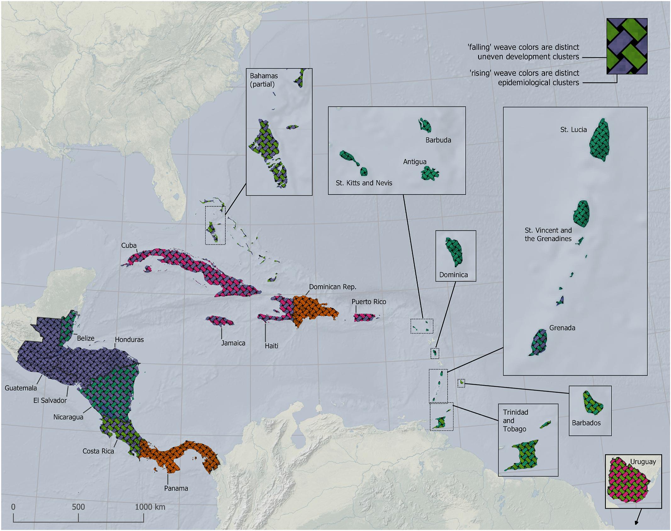
from Chaves LF, MD Friberg, LA Hurtado, R Marín Rodríguez, D O’Sullivan, and LR Bergmann. 2021 (online first). Trade, uneven development and people in motion: Used territories and the initial spread of COVID-19 in Mesoamerica and the Caribbean. Socio-Economic Planning Sciences.
A key aspect is the way that strands in the weave link across boundaries, and the way that directionality in the pattern allows distinct patterns in more than one attribute to be simultaneously viewed.
This map was done with SVG symbol fills in QGIS, and was (very!) fiddly to produce. Nevertheless we thought the general idea has merit and decided to develop it further
Motivation and other approaches
Increasingly, we deal with highly multivariate data. Many approaches can be used to visualise such data spatially, and we consider a few below.
Small multiples
This is sf’s default plot output for a dataset.
plot(region)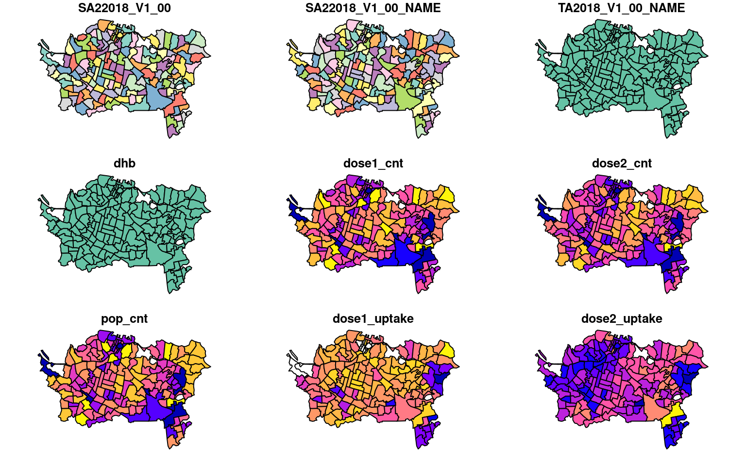
Small multiples can be effective, but require cross-comparison by eye among multiple, perhaps detailed, and necessarily small maps. They need a lot of screen or paper real estate.
Bivariate choropleths
This idea has been around for over 50 years, yet remains hard to execute well, e.g., using Jan Caha’s QGIS plugin which implements an approach described by Joshua Stevens in this post.
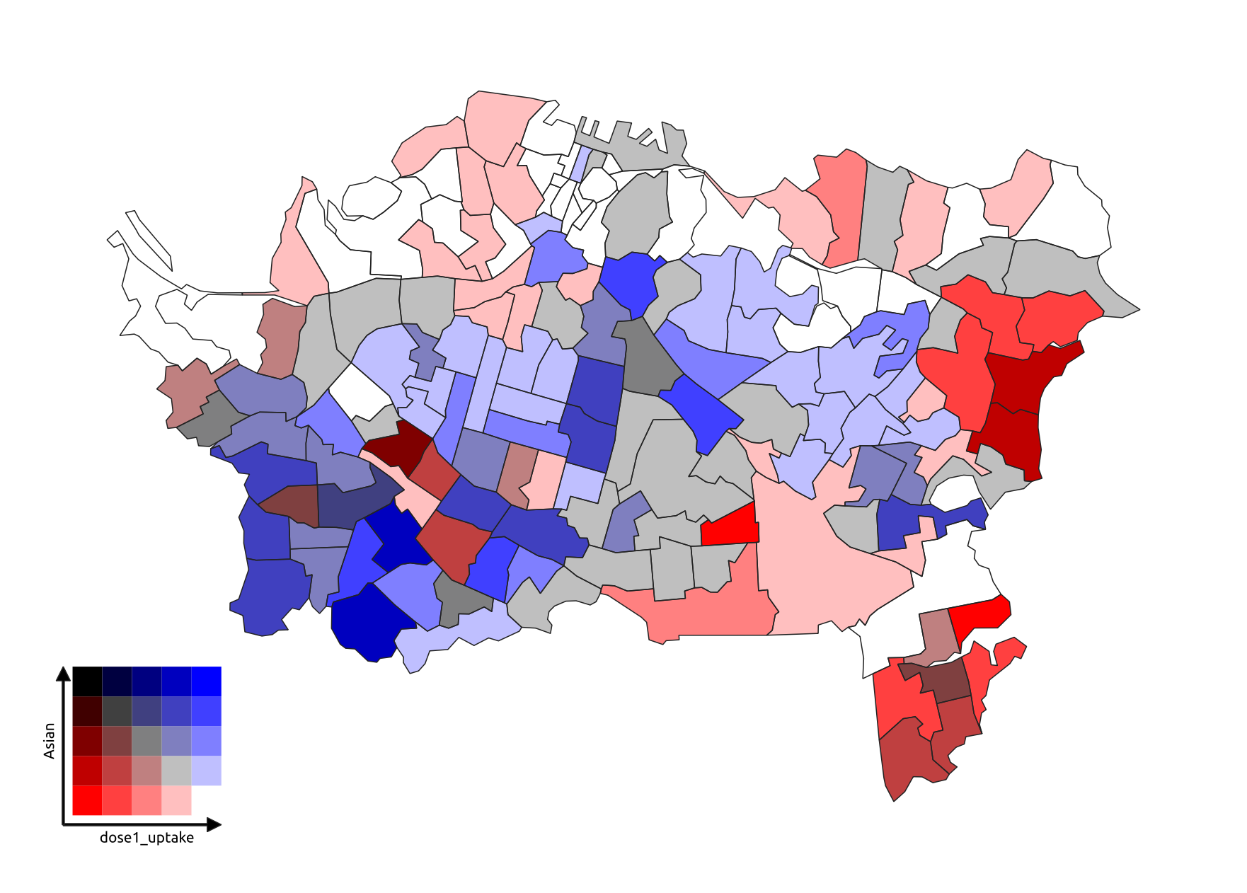
Bivariate choropleth made in QGIS
Of course the method is limited to two colours.
Trivariate choropleths
Mixing three colours is hard, but e.g., the tricolore package can do this…
eth_mix <- tricolore::Tricolore(
region, p1 = "pEuropean", p2 = "pMaori", p3 = "pAsian", breaks = 5
)
region$eth_mix_tri <- eth_mix$rgb
ggplot(region) +
geom_sf(aes(fill = eth_mix_tri)) +
scale_fill_identity() +
annotation_custom(
grob = ggplotGrob(eth_mix$key + labs(L = 'Pākehā', T = 'Māori', R = 'Asian')),
xmin = 1.7465e6, xmax = 1.7535e6, ymin = 5.9075e6, ymax = 5.9125e6)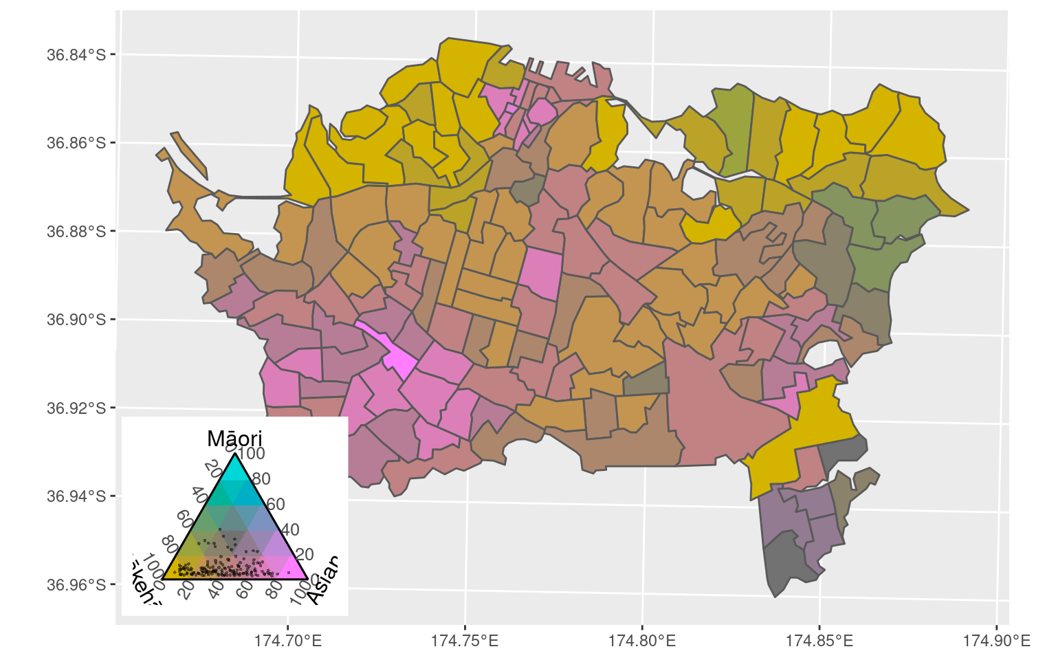
The problem is that blends of three colours have a tendency to all end up muddy browns!
Symbols over choropleths
A straightforward option is to display small statistical graphics, such at time series, histograms, pie charts, box plots on top of a standard map view. Here’s an example made in QGIS.
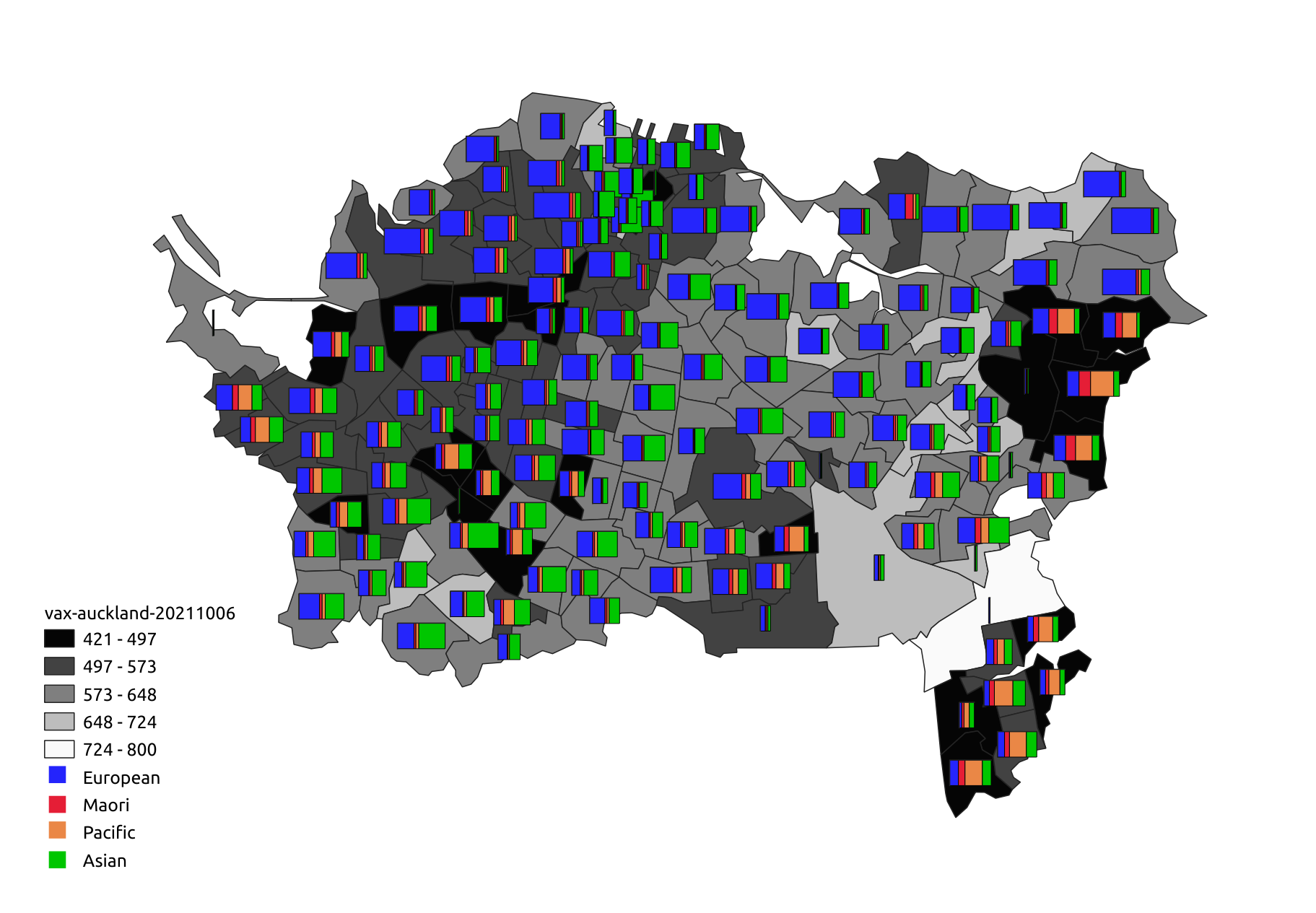
Choropleth with symbols made in QGIS
Multivariate symbols
The classic example is Dorling’s Chernoff faces map of the UK 1987 election.

Figure 8.10 Dorling D. 2012. The visualisation of spatial social structure. Chichester, England: John Wiley & Sons.
This example combines a cartogram representation for location of the constituencies, coloured according to a trivariate scheme, with four additional variables represented in the face symbols.
Multi-element patterns
There are many variations on this idea, but perhaps the most common is a categorical dot map. The example below was made using tmap and data preparation code from James Smythe’s cultureofinsight blog
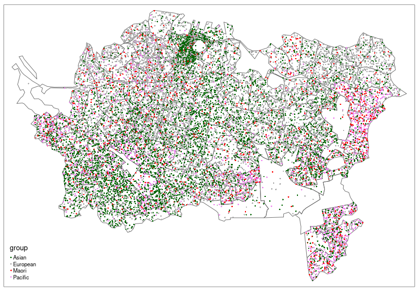
dot map of ethnic composition
Here each dot represents ~25 people and colours represent different census-classified ethnicities. This approach can be very effective (see for example the Cooper Center’s Racial Dot Map), although great care is required in placing—and in interpreting the placement of—the dots
This last approach is closest in spirit to ours, as it seeks to allow the different symbolisations to be seen together and also partly dissolves the polygon boundaries that underpin the data.
A woven map
Below we show a woven map and the code that produced it.
Our code allows a weave unit in sf format to be constructed (more on these later), and then applied using a weave_layer() function to create a weave layer (here, the variable fabric, with an attribute strand identifying each strand in the weave
weave_unit <- get_biaxial_weave_unit(spacing = 200, type = "twill", n = 3,
aspect = 0.6, strands = "ab|cd",
crs = st_crs(region))
fabric <- weave_layer(weave_unit, region, angle = 30)We can split the data by id attribute of fabric to make symbolising them independently easier
layers <- fabric %>% split(as.factor(fabric$strand))Below we make the map using the tmap package but this could be done in any GIS-adjacent tool since the weave layer is a standard geospatial dataset, not a graphical overlay
tm_shape(region, name = "Dose 2 uptake") +
tm_fill(col = "dose2_uptake", palette = "inferno", style = "cont",
title = "Dose 2 per 1000", id = "SA22018_V1_00_NAME") +
tm_shape(layers$a, name = "Pākehā") +
tm_fill(col = "pEuropean", palette = "Greys", title = "% Pākehā", n = 3,
id = "SA22018_V1_00_NAME", popup.vars = c("pEuropean")) +
tm_shape(layers$b, name = "Māori") +
tm_fill(col = "pMaori", palette = "Reds", title = "% Māori", n = 3,
id = "SA22018_V1_00_NAME", popup.vars = c("pMaori")) +
tm_shape(layers$c, name = "Pasifika") +
tm_fill(col = "pPacific", palette = "Purples", title = "% Pasifika", n = 3,
id = "SA22018_V1_00_NAME", popup.vars = c("pPacific")) +
tm_shape(layers$d, name = "Asian") +
tm_fill(col = "pAsian", palette = "Greens", title = "% Asian", n = 3,
id = "SA22018_V1_00_NAME", popup.vars = c("pAsian"))Implementing woven maps
Our implementation is conceptually straightforward:
A weave unit ‘tile’ is generated and replicated and tiled across a regular rectangular or hex grid of points generated by geospatial tools (here we use sf::st_make_grid
We can also affine transform (skew, magnify, rotate, etc) the weave by applying the inverse transform to the map area before doing the tiling, then inverting the transformations

tiling a weave unit
The question is: “What repeatable units can tile across such grids to give the appearance of a woven pattern?”
It turns out this has been of interest to mathematicians (Grünbaum and Shephard 1985, 1986), who call such tileable elements the fundamental blocks (‘tiles’) of isonemal fabrics (weave patterns)
Our proof-of-concept R tools follow this sequence to make weave patterns:
- Make a weave unit
- Tile the map area with the weave unit
- Export to a multi-layer GPKG
- Symbolise the weave elements as desired in any tool
Weave units (or fundamental blocks)
We have implemented a wide range of weave units, both biaxial and triaxial
Biaxial weaves
We generate biaxial weave units using a matrix multiplication method (see Glassner 2002)
Plain weaves
Traditional over-under weave patterns with threads in two directions, the warp (north-south!) and the weft (east-west!)
Simplest is a plain weave
rect11_unit <- ## plain weave example
get_biaxial_weave_unit(spacing = 300, type = "plain",
strands = "a|b", crs = st_crs(region))
rect11_unit$primitive %>% plot(border = NA, main = "Plain weave unit")
This will produce a checkerboard pattern when tiled
The colours are not the final colours that would be applied to a map, but denote map areas that would be symbolised differently
This simple pattern could be useful if clearly distinct palettes were used in the warp and weft elements
More useful is if we change the aspect of the weave unit elements so that we can distinguish directions
rect11_unit <- ## plain weave example
get_biaxial_weave_unit(spacing = 300, aspect = 0.8,
strands = "a|b", crs = st_crs(region))
rect11_unit$primitive %>% plot(border = NA, main = "Plain weave unit, with directions")
More threads, more colours
The weave is highly customisable
We can add more unique strands in either or both directions
This unit might be used to map 5 attributes
rect32_unit <-
get_biaxial_weave_unit(spacing = 300, aspect = sqrt(0.5),
strands = "abc|de", crs = st_crs(region))
rect32_unit$primitive %>% plot(border = NA, main = "Plain weave, 3 warp and 2 weft colours")
Missing threads
We can even leave gaps or duplicate threads
rect34_unit <- ## plain weave example
get_biaxial_weave_unit(spacing = 150, aspect = 0.8,
strands = "ab-|cc-d", crs = st_crs(region))
rect34_unit$primitive %>% plot(border = NA, main = "Complex plain weave with missing strands")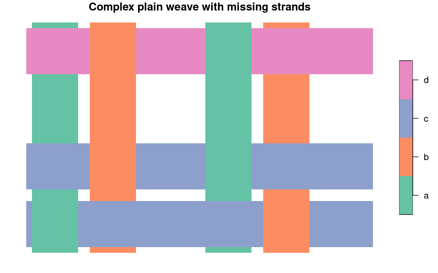
Twill weaves and basket weaves
There are many different weave patterns
In twill weaves an over-under pattern (here 2-2) shifts one strand between consecutive weft strands to produce a distinctive diagonal pattern
twill_unit <-
get_biaxial_weave_unit(spacing = 150, type = "twill", n = c(2, 2),
aspect = 0.7, strands = "a|b", crs = st_crs(region))
twill_unit$primitive %>% plot(border = NA, main = "2 over 2 under twill weave")
In basket weaves, an over-pattern repeats between consecutive weft strands to give a checkerboard appearance, but note that more than one colour might be applied in either or both directions
basket_unit <-
get_biaxial_weave_unit(spacing = 150, type = "basket", n = 2,
aspect = 0.7, strands = "ab|cd", crs = st_crs(region))
basket_unit$primitive %>% plot(border = NA, main = "2 over 2 under basket weave")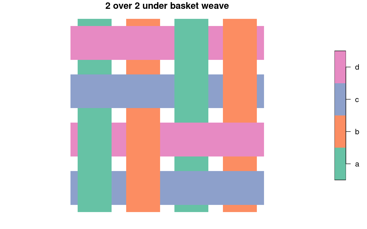
Other weaves
Because we are using a matrix multiplication approach, we can generate any biaxial weavable pattern, even crazy ones, like this:
this_unit <-
get_biaxial_weave_unit(spacing = 37.5, type = "this", strands = ids,
crs = st_crs(region))
this_unit$primitive %>% plot(border = NA, main = "Pattern from Glassner 2002")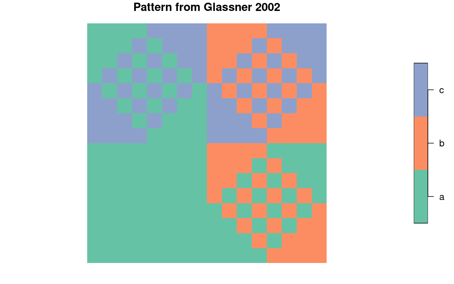
Triaxial weaves
We’ve made less progress (so far) with triaxial weaves, largely because we have yet to figure out a flexible underlying representation and instead are relying on ‘pure geometry’
Hexagonal
This weave has strands running in 3 directions, and uses a hexagonal tiling
We can ‘split’ strands along their length to allow more attributes
hex_unit <- ## hex example
get_triaxial_weave_unit(spacing = 600, margin = 2,
strands = "a|bc|def", type = "hex", crs = st_crs(region))
hex_unit$tile %>% plot(col = "white", border = "black",
main = "Hex-based triangular weave")
hex_unit$primitive %>% plot(border = NA, add = TRUE)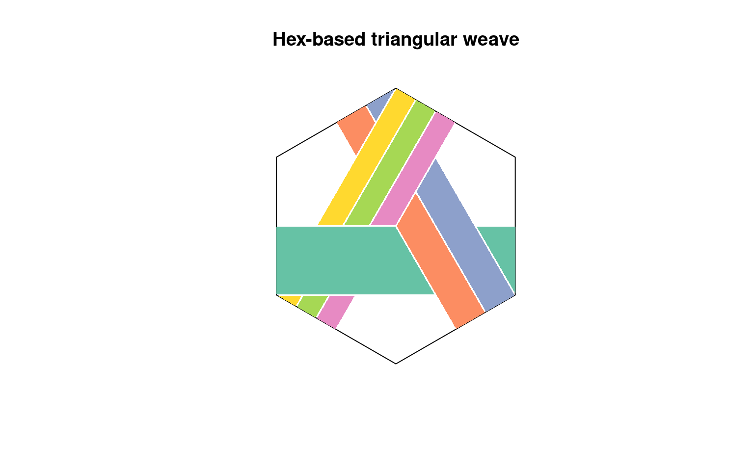
A cube is another option (sometimes called ‘madweave’)
This produces some odd 3D effects when tiled (see below)
cube_unit <-
get_triaxial_weave_unit(spacing = 600, strands = "ab|cd|ef", margin = 2,
type = "cube", crs = st_crs(region))
cube_unit$primitive %>% plot(border = NA,
main = "Mad weave (so called) with two colours in each direction")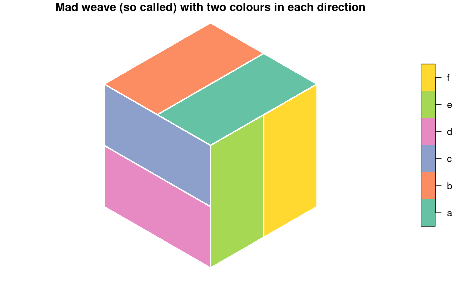
Diamond
An alternative way to produce a triangular weave is with a diamond repeating unit with angles 60° and 120°
diamond_unit <- ## diamond example
get_triaxial_weave_unit(spacing = 600, margin = 2,
strands = "a|b|c", type = "diamond", crs = st_crs(region))
diamond_unit$tile %>% plot(col = NA, border = "black",
main = "Triangular weave with a diamond fundamental block")
diamond_unit$primitive %>% plot(border = NA, add = TRUE)
Weave a map
As another example here are some data from Ellis et al. 2021, which aim to show change over 1000s of years in human-affected regions they designate as anthromes
First, a small multiple approach
anthromes <- st_read("data/nz-anthromes-dgg.gpkg")
tmap_mode("plot")
tm_shape(anthromes) +
tm_fill(col = paste("class", seq(2000, 1800, -100), sep = ""),
palette = anthrome_colors(), title = "Anthrome") +
tm_layout(panel.labels = c("2000", "1900", "1800"),
legend.outside = TRUE)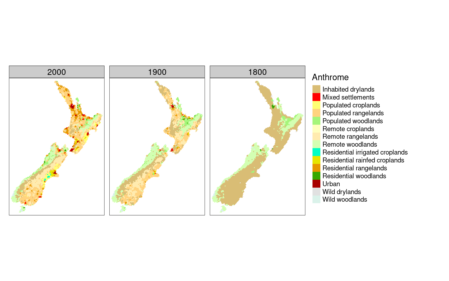
And now we make a weave unit and tile it so we can put three snapshots in a single map
tri_unit <- get_triaxial_weave_unit(spacing = 8000, strands = "a|b|c", type = "hex",
crs = st_crs(anthromes))
fabric2 <- weave_layer(tri_unit, anthromes, angle = 15)Some tidying up is needed for the web map hover labelling (we need to make this easier to carry out as part of the weave_layer() function)
fabric2 <- st_read("data/fabric2-raw.gpkg") %>%
mutate(label = if_else(strand == "a",
paste("1800", class1800), # make labels including
ifelse(strand == "b", # year and anthrome
paste("2000", class2000),
paste("1900", class1900)))) %>%
select(21, 1:19) # put them in 1st column
layers2 <- fabric2 %>% split(as.factor(fabric2$strand))
tmap_mode("view")The map itself is simple enough to make in tmap
tm_shape(layers2$a, name = "1800") +
tm_fill(col = "class1800", palette = anthrome_colors(), legend.show = FALSE) +
tm_shape(layers2$c, name = "1900") +
tm_fill(col = "class1900", palette = anthrome_colors(), legend.show = FALSE) +
tm_shape(layers2$b, name = "2000") +
tm_fill(col = "class2000", palette = anthrome_colors(), title = "Anthrome")