
Paul Klee’s Polyphony 1932, Kunstmuseum, Basel
image source commons.wikimedia.org
Orange cranberry cake by
Helen Fletcher on
flickr.com
image Ian McHarg's Design with Nature 1969
source suzanneodonovan.wordpress.com
Makara turbines from Hawkins Hill
image source gitta.info
st_intersection in R
Overlay of factors indicative of low
quality housing Richmond, Virginia, 1934,
in Overlay (in GIS) article by Ola Ahqvist
in International Encyclopedia of Human
Geography
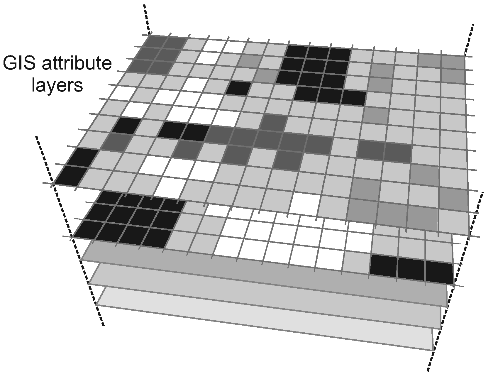
r3 <- r1 + r2image source gis.stackexchange.com
aerial view of the Arc de Triomphe, Paris
image source yatzer.com
image source commons.wikimedia.org
image source flickr by Tony Hisgett
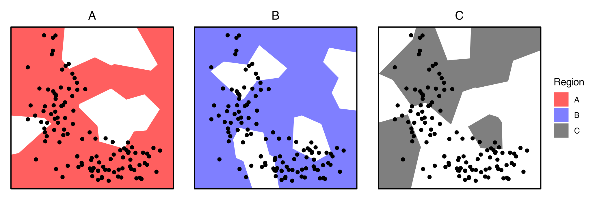
                    Region     n  area in_density out_density weight  log_w
                    <chr>  <int> <dbl>      <dbl>       <dbl>  <dbl>  <dbl>
                  1 A        109 0.891      122.         25.1  4.87   0.688
                  2 B         82 0.921       89.0       121.   0.735 -0.134
                  3 C         38 0.525       72.4       115.   0.628 -0.202
Francis Galton’s illustration of correlation, 1875 image source commons.wikimedia.org