library(sf)
library(ggplot2)
library(rnaturalearth)
library(dplyr)

n <- 2500There isn’t as much land near the poles, so how do you make uniform randomly distributed points in lat-lng coordinate space. Here’s how!
Needed libraries are the usual suspects plus rnaturalearth for basemap data
The key thing to realise here is that random uniform numbers in both latitude and longitude will not be evenly distributed on Earth’s surface, because the meridians converge toward the poles. We can make two datasets to show this. First a naive set of randomly located points:
pts_naive <- data.frame(lon = runif(n) * 360 - 180,
                        lat = runif(n) * 180 - 90,
                        type = "naive")
Here comes the science…
And now a set where inserting a cosine correction ensures that the distribution of latitudes is appropriately more dense close to the equator:
pts_even <- data.frame(lon = runif(n) * 360 - 180,
                       lat = acos(runif(n) * 2 - 1) * 180 / pi - 90,
                       type = "even")
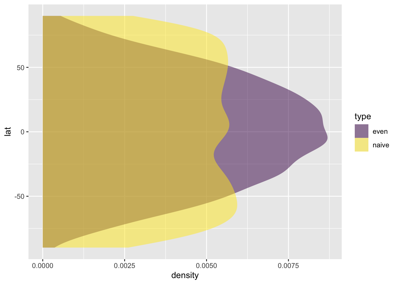
Compare the latitude distributions
We can make up a combined data table and directly compare the distribution of the latitudes with a nice density plot. The increased representation of points in the mid-latitudes with the cosine correction is clear.
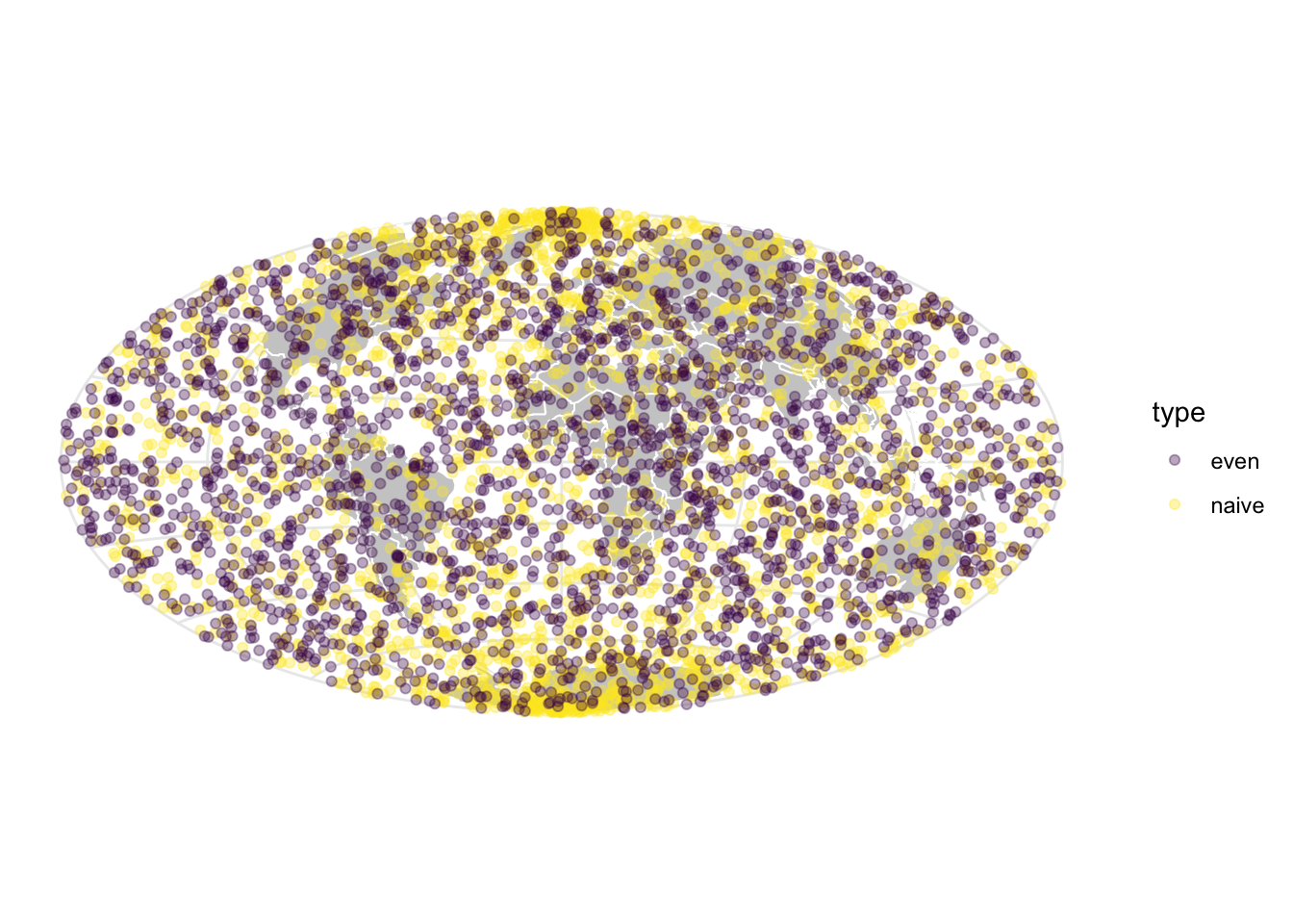
Make a map
Use an equal-area projection to clearly see the problem geographically.
w <- ne_countries(returnclass = "sf") |>
  st_transform("+proj=hammer")

pts_sf <- pts |>
  st_as_sf(coords = 1:2, crs = 4326)

ggplot(w) +
  geom_sf(fill = "#cccccc", colour = "white", lwd = 0.35) +
  geom_sf(data = pts_sf, aes(colour = type), alpha = 0.35) +
  scale_colour_viridis_d() +
  theme_minimal()
The naively distributed points are clearly denser at the poles than they should be, where the cosine term in the ‘even’ points generation method makes them evenly distributed over the globe.


