library(akima)
library(tidyr)
library(dplyr)
library(ggplot2)
library(sf)Load libraries
This notebook shows how we can use a set of paired ‘control points’ of a projection to interpolate unknown locations to that projection. The basic setup is a table of pairs of coordinate pairs \((x_1,y_1)\) and \((x_2,y_2)\) representing the same location in two different coordinate systems. Given this setup assuming that the projection is well-behaved with no serious ‘breaks’ we can form an empirical projection to estimate locations in one coordinate system for ‘unknown’ locations in the other. See, for example
- Gaspar J A, 2011, “Using Empirical Map Projections for Modeling Early Nautical Charts”, in Advances in Cartography and GIScience Ed A Ruas (Springer Berlin Heidelberg), pp 227–247, http://link.springer.com/10.1007/978-3-642-19214-2_15
Get input datasets
The empirical projection
This file contains points on a global grid system, generated using the dggridR package. We can see the points in ‘lat-lon’ space below. Note how because this is a global grid system the points appear to ‘thin out’ towards the poles. This is an artifact of plotting the points in lat-lon, which is also explored in this post.
emp_proj <- read.csv("dgg-2432-no-offsets-p4-briesemeister.csv")
ggplot(emp_proj) +
  geom_point(aes(x = lon, y = lat), size = 0.05) +
  coord_equal()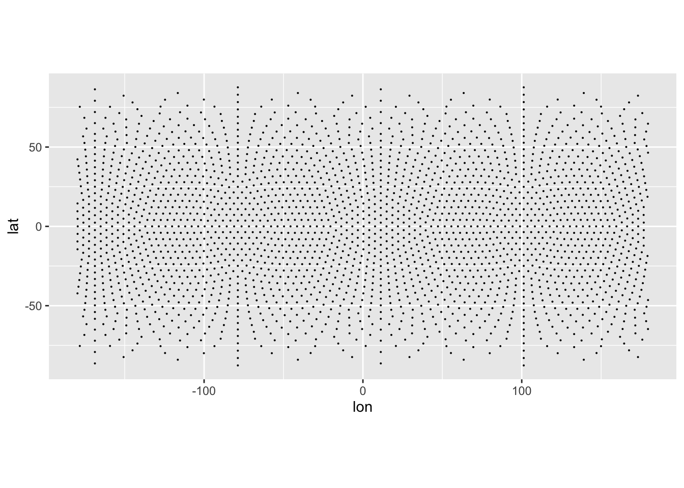
Inspection of the data shows we have two sets of coordinates lon, lat and x, y.
head(emp_proj) ID dir lon lat x y
1 0 . 11.25 58.28253 -428675.9 1520344
2 1 . -168.75 58.28253 -1197290.8 7794188
3 2 . -168.75 65.09003 -1120150.7 7234575
4 3 . -168.75 72.07407 -1048583.9 6613223
5 4 . -168.75 79.18998 -973499.6 5945572
6 5 . -168.75 86.38746 -892969.4 5242144This projection is Briesemeister, which is an oblique form of the Hammer-Aitoff projection. See
- Briesemeister W, 1953, “A New Oblique Equal-Area Projection” Geographical Review 43(2) 260
It’s possible to form this projection with a proj string, but it is not commonly supported in GIS, and who knows proj strings that well?! For the record, this is the string you are looking for:
+proj=ob_tran +o_proj=hammer +o_lat_p=45 +o_lon_p=-10 +lon_0=0 +R=6371007A sample dataset
We also want a set of points to project, and what better than a world map. Note that we can only project points, so this is points along world coastlines, not polygons.
pts <- read.csv("world_better.csv") |>
  dplyr::select(lon, lat)

# sanity check with a map
ggplot(pts) +
  geom_point(aes(x = lon, y = lat), size = 0.05) +
  coord_equal()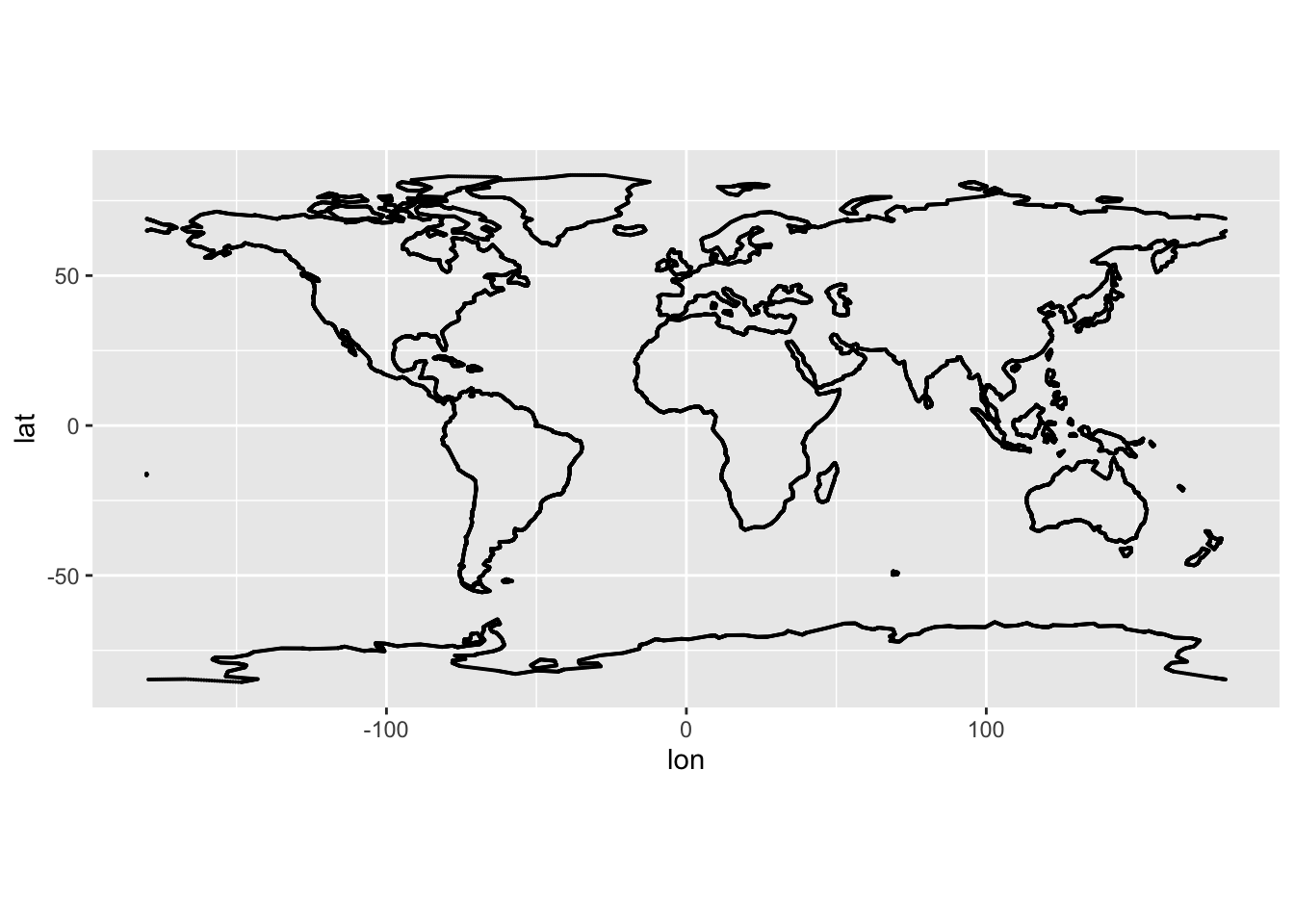
Triangles interpolator
There are many different ways we can do this kind of interpolation. The simplest is based on triangulation. This method is available in the package interp but also in akima which is much quicker. The output x and y coordinates are formed by interpolating as shown below. x and y are the known locations of the input coordinate, which here are the longitude and latitude in out empirical projection dataset emp_proj. The desired outputs are at the longitude and latitude coordinates in the world maps dataset pts. And we do the interpolation twice, once for the x coordinate and once for the y coordinate in our target projection.
x_out <- akima::interpp(x = emp_proj$lon, y = emp_proj$lat, z = emp_proj$x,
                xo = pts$lon, yo = pts$lat)
y_out <- akima::interpp(x = emp_proj$lon, y = emp_proj$lat, z = emp_proj$y,
                xo = pts$lon, yo = pts$lat)
Now make up a results data table and map it. akima puts the result in a column z in its output.
result <- data.frame(x = x_out$z, y = y_out$z)
ggplot(result) +
  geom_point(aes(x = x, y = y), size = 0.05) +
  coord_equal()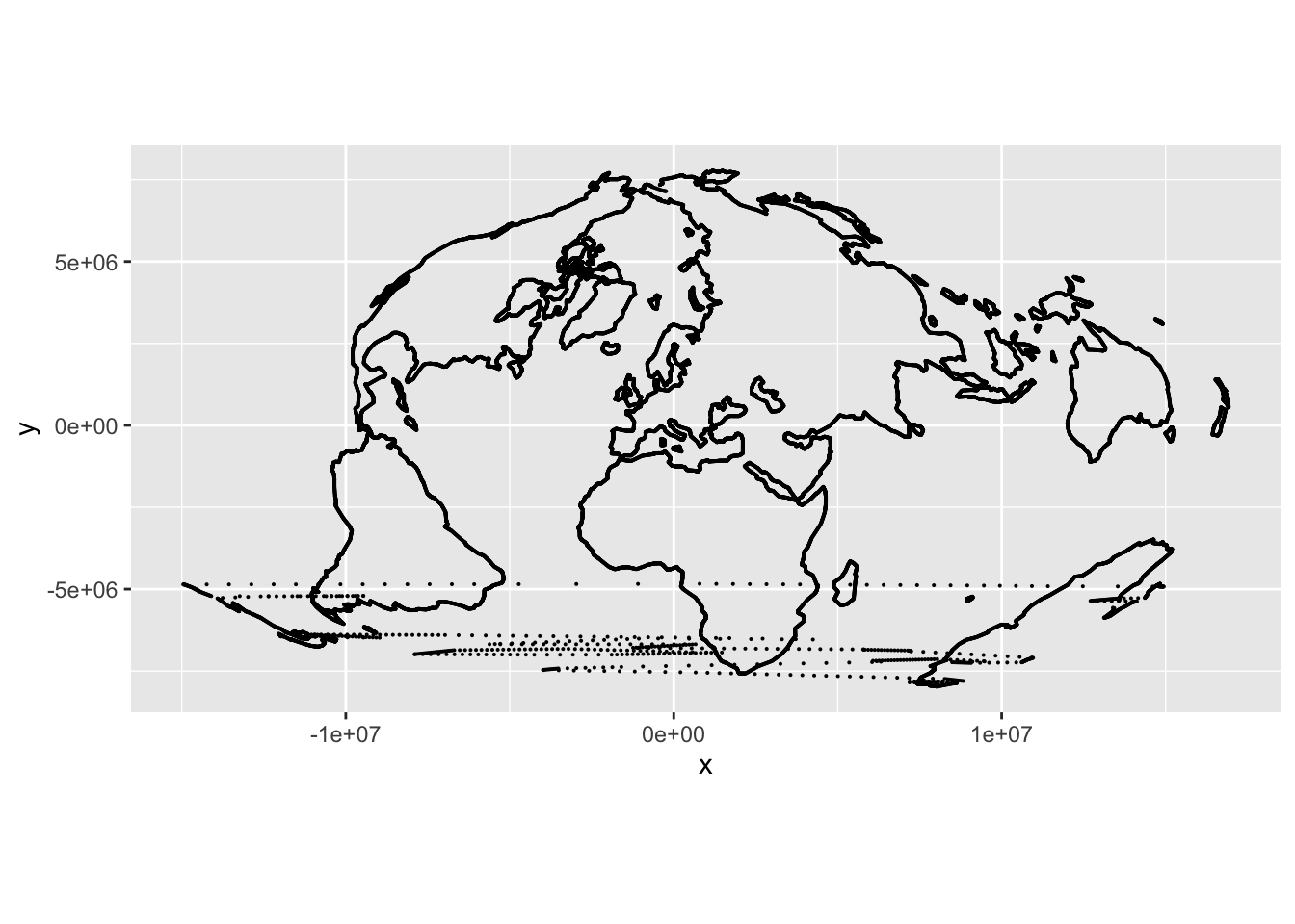
Apply the empirical projection’s cut region
What are those dots across the southern area of the map? These are points that happen to fall in triangles in the first coordinate system (i.e. lon-lat) where one corner of the triangle lies on a different side of a discontinuity in the projection than the other corners. We should avoid projecting points inside these triangles because they project (as we can see!) unreliably.
For the Briesemeister projection we know the precise location of this discontinuity, and have prepared a file delineating the ‘cut’ position. We can use this to remove points from the sample dataset that lie inside triangles that intersect the cut region.
First, here is the discontinuity. Points close to or on this line could end up in very different parts of the projected output and so are ‘unsafe’ to project using our interpolation-based approximation.
cut_sf <- st_read("briesemeister-cut.geojson")Reading layer `briesemeister-cut' from data source
`/Users/david/Documents/code/dosull.github.io/posts/2021-10-21-experiments-with-r-interpolators/briesemeister-cut.geojson'
using driver `GeoJSON'
Simple feature collection with 1 feature and 0 fields
Geometry type: LINESTRING
Dimension: XY
Bounding box: xmin: -179.8892 ymin: -82.94613 xmax: -0.3442386 ymax: 44.55223
Geodetic CRS: WGS 84ggplot(cut_sf) +
geom_sf()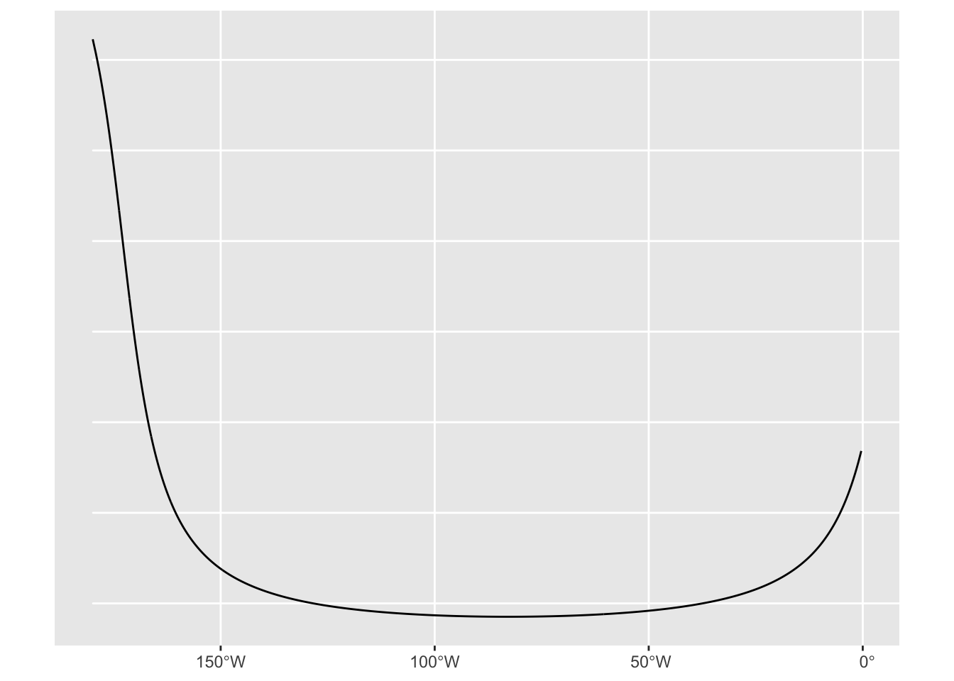
Now triangulate the empirical projection data points, and assemble a polygon from all those triangles that are intersected by the discontinuity.
# make the cut region into a sf dataset
emp_proj_sf <- emp_proj |>
  st_as_sf(coords = c("lon", "lat")) |>
  st_set_crs(4326)

triangles <- emp_proj_sf |>
  st_union() |>
  st_triangulate() |>   # triangulation of empirical projection points
  st_cast() |>
  st_as_sf()

cut_triangles <- triangles |>
  st_filter(cut_sf)

cut_region_sf <- cut_triangles |>
  st_filter(cut_sf) |>
  st_union() |>
  st_as_sf()
We quite reasonably get a warning that triangulation doesn’t really apply to geographical coordinates, but… akima did the interpolation by triangulating these points and it doesn’t know it’s unsafe (because it’s not a geospatial package). It’s not actually ‘unsafe’ as such in this case, because we aren’t using the triangulation for its metric properties anyway. So… we ignore this warning and plot this to see what we are dealing with
ggplot(triangles) +
  geom_sf(colour = "grey") +
  geom_sf(data = cut_triangles, fill = "grey", colour = "white") +
  geom_sf(data = cut_region_sf, fill = "#00000000", colour = "black") +
  geom_sf(data = cut_sf, color = "red")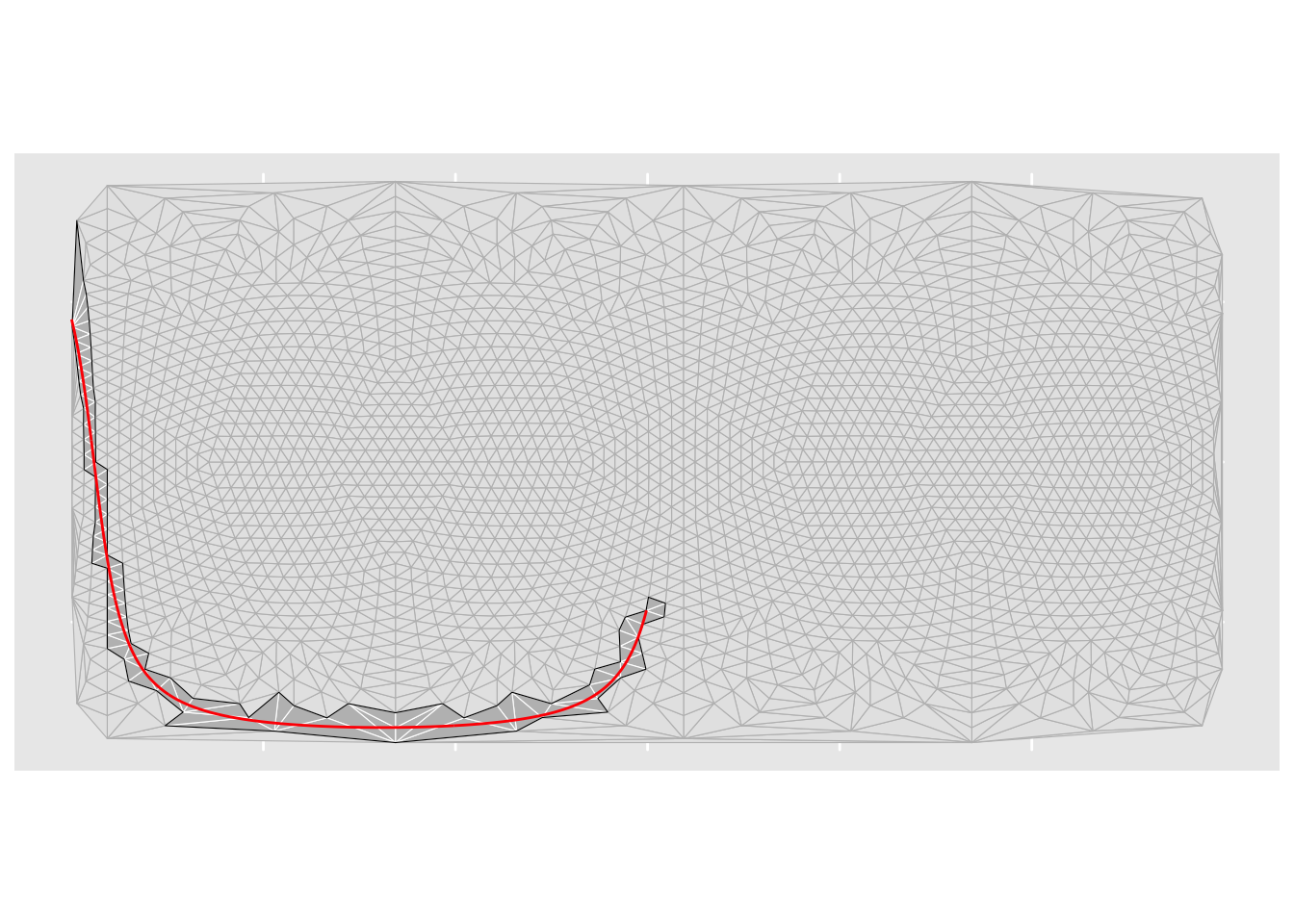
Now we use st_disjoint to remove points in the data to project that are inside the cut region.
pts_to_project_sp <- pts |>
  st_as_sf(coords = c("lon", "lat")) |>
  st_set_crs(4326) |>
  st_filter(cut_region_sf, .predicate = st_disjoint) |>
  as("Spatial")
The last step converts the points to the SpatialPointsDataFrame format of the sp package, which akima can also work with:
# we also need the empirical projection data in the sp format
emp_proj_sp <- emp_proj_sf |>
  as("Spatial")

x <- akima::interpp(emp_proj_sp, z = c("x"), xo = pts_to_project_sp, linear = TRUE)
y <- akima::interpp(emp_proj_sp, z = c("y"), xo = pts_to_project_sp, linear = TRUE)
A bit unexpectedly, akima outputs the data to a two column dataframe with the interpolated values in a column with the same name as the input data, so getting the results into a final output table is as below.
result <- data.frame(x = x$x, y = y$y)
ggplot(result) +
  geom_point(aes(x = x, y = y), size = 0.05) +
  coord_equal()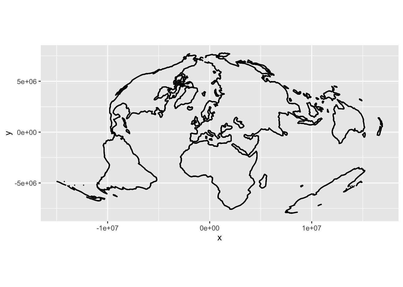
And those rogue dots are all gone!
![]()