library(sf)
library(tmap)
library(spatstat)
library(raster)
library(dplyr)Packages
This requires a surprising number of moving parts (at least the way I did it):
Data
The data are some point data (Airbnb listings from here) and some polygon data (NZ census Statistical Area 2 data).
Load the data
polys <- st_read("sa2.gpkg")Reading layer `sa2' from data source
`/Users/david/Documents/code/dosull.github.io/posts/2021-10-21-kde/sa2.gpkg'
using driver `GPKG'
Simple feature collection with 78 features and 5 fields
Geometry type: MULTIPOLYGON
Dimension: XY
Bounding box: xmin: 1735096 ymin: 5419590 xmax: 1759041 ymax: 5443768
Projected CRS: NZGD2000 / New Zealand Transverse Mercator 2000pts <- st_read("abb.gpkg")Reading layer `abb' from data source
`/Users/david/Documents/code/dosull.github.io/posts/2021-10-21-kde/abb.gpkg'
using driver `GPKG'
Simple feature collection with 1254 features and 16 fields
Geometry type: POINT
Dimension: XY
Bounding box: xmin: 1742685 ymin: 5420357 xmax: 1755385 ymax: 5442630
Projected CRS: NZGD2000 / New Zealand Transverse Mercator 2000And have a look
tm_shape(polys) +
  tm_polygons() +
  tm_shape(pts) +
  tm_dots()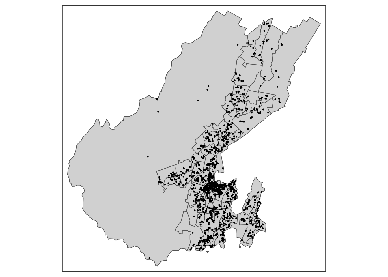
spatstat for density estimation
The best way I know to do density estimation in the R ecosystem is using the spatstat library’s specialisation of base R’s density function. That means converting the point data to a spatstat planar point pattern (ppp) object, which involves a couple of steps.
pts.ppp <- pts$geom %>%
  as.ppp()
A point pattern also needs a ‘window’, which we’ll make from the polygons.
pts.ppp$window <- polys %>%
  st_union() %>%       # combine all the polygons into a single shape
  as.owin()            # convert to spatstat owin - again maptools...
Now the kernel density
We need some bounding box info to manage the density estimation resolution
bb <- st_bbox(polys)
cellsize <- 100
height <- (bb$ymax - bb$ymin) / cellsize
width <- (bb$xmax - bb$xmin) / cellsize
Now we specify the size of the raster we want with dimyx (note the order, y then x) using height and width.
We can convert this directly to a raster, but have to supply a CRS which we pull from the original points input dataset. At the time of writing (August 2021) you’ll get a complaint about the New Zealand Geodetic Datum 2000 because recent changes in how projections and datums are handled are still working themselves out.
kde <- density(pts.ppp, sigma = 500, dimyx = c(height, width)) %>%
  raster()
crs(kde) = st_crs(pts)$wkt  # a ppp has no CRS information so add it
Let’s see what we got
We can map this using tmap.
tm_shape(kde) +
  tm_raster(palette =  "Reds")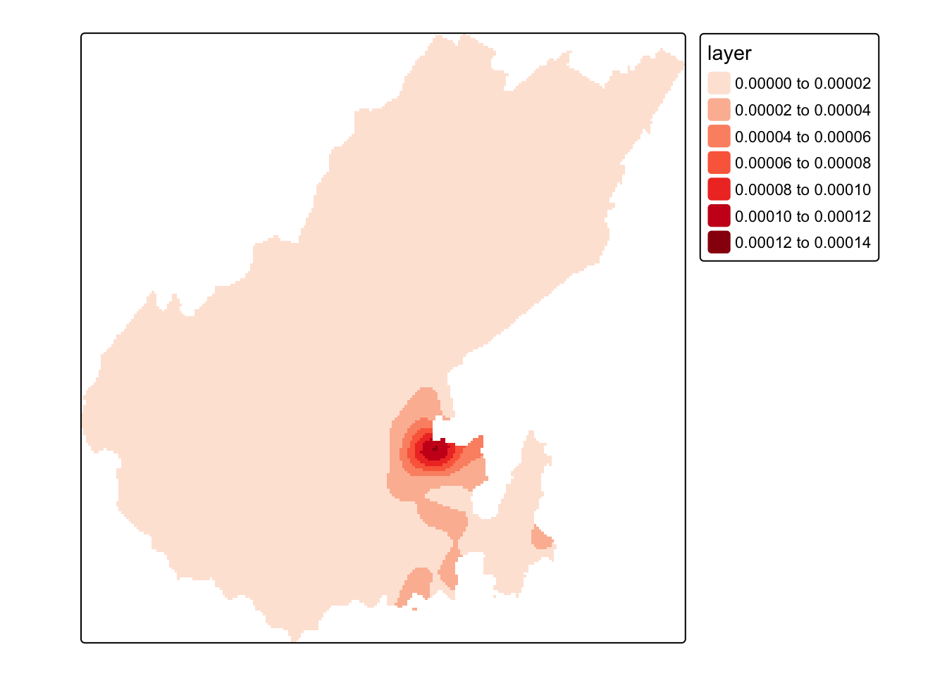
A fallback sanity check
To give us an alternative view of the data, let’s just count points in polygons
polys$n <- polys %>%
  st_contains(pts) %>%
  lengths()
And map the result
tm_shape(polys) +
  tm_polygons(col = "n", palette = "Reds", title = "Points in polygons")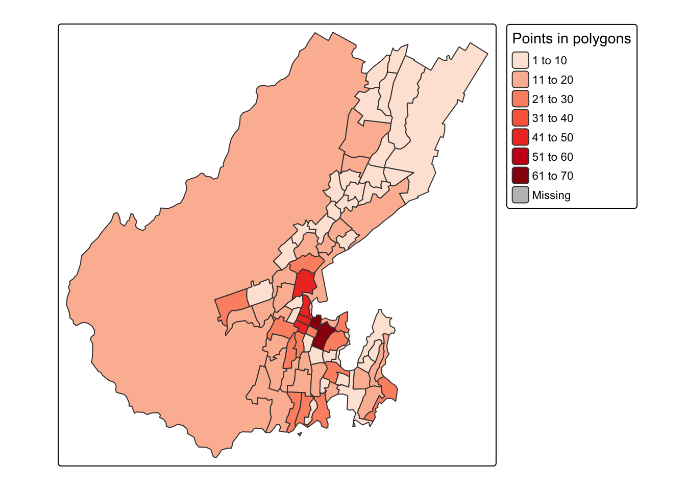
Aggregate the density surface pixels to polygons
This isn’t at all necessary, but is also useful to know. This is also a relatively slow operation. Note that we add together the density estimates in the pixels contained by each polygon.
summed_densities <- raster::extract(kde, polys, fun = sum)Append this to the polygons and rescale so the result is an estimate of the original count. We multiply by cellsize^2 because each cell contains an estimate of the per sq metre (in this case, but per sq distance unit in general) density, so multiplying by the area of the cells gives an estimated count.
polys$estimated_count = summed_densities[, 1] * cellsize ^ 2And now we can make another map
tm_shape(polys) +
  tm_polygons(col = "estimated_count", palette = "Reds",
              title = "500m KDE summed")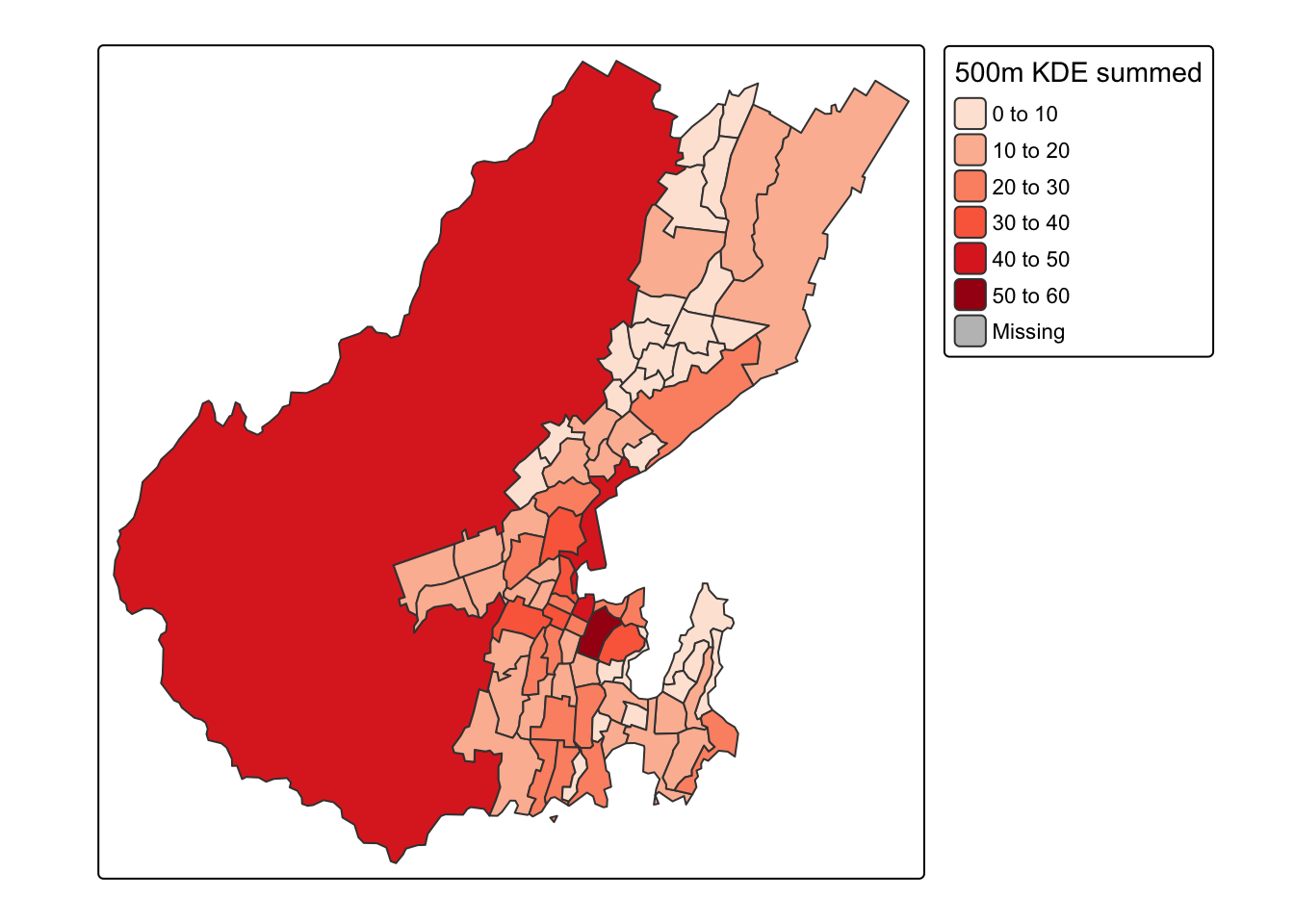
Spot the deliberate mistake?!
Something doesn’t seem quite right! What’s with the large numbers in the large rural area to the west of the city? Thing is, you shouldn’t really map count data like this, but should instead convert to densities. If we include that option in the tm_polygons function, then order is restored.
tm_shape(polys) +
  tm_polygons(col = "estimated_count", palette = "Reds", convert2density = TRUE,
              title = "500m KDE estimate")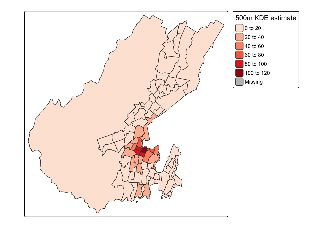
Really, this should be done with the earlier map of points in polygons too, so let’s show all three side by side. tmap_arrange is nice for this, although it has trouble making legend title font sizes match, unless you do some creative renaming. I’ve also multiplied the KDE result by 1,000,000 to convert the density to listings per sq. km, and we can see that the three maps are comparable.
m1 <- tm_shape(kde * 1000000) +
  tm_raster(palette = "Reds", title = "500m KDE")
m2 <- tm_shape(polys) +
  tm_fill(col = "n", palette = "Blues", convert2density = TRUE,
              title = "Point density")
m3 <- tm_shape(polys) +
  tm_fill(col = "estimated_count", palette = "Greens", convert2density = TRUE,
              title = "KDE summed")
tmap_arrange(m1, m2, m3, nrow = 1)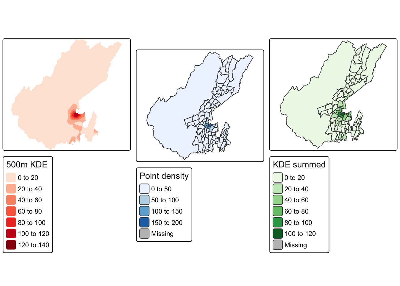
![]()