knitr::opts_chunk$set(error = TRUE, message = TRUE)

Packages

library(sf)
library(tmap)
library(dplyr)
library(wk)

sf::sf_use_s2(FALSE)

A simple square

Just to get things set up let’s make a simple square.

square <- (st_polygon(list(matrix(c(-1, -1, 1, -1, 1, 1, -1, 1, -1, -1), 
                                 5, 2, byrow = TRUE))) * 0.5 + c(1, 0)) %>%
  st_sfc()

tm_shape(square) + 
  tm_borders(col = "red") + 
  tm_grid()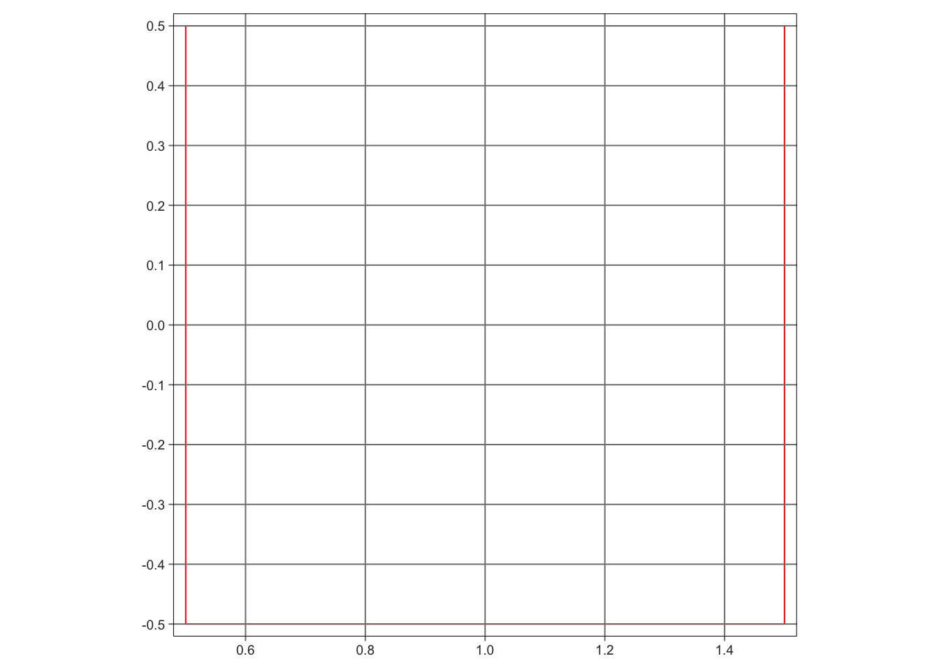

Warning: Currect projection of shape square unknown. Long-lat (WGS84) is
assumed.

Simple transformations

In the code above, we made a polygon and multipled it by 0.5, then added c(1,0) to it. This had the effect of scaling it by 0.5 andthen translating it by the vector \[\left[\begin{array}{c}1\\0\end{array}\right]\]

These unlikely looking operations are perfectly valid, although they feel a bit ‘off’.

Even more unlikely is that you can multiply an sf object by a matrix…

ang <- pi / 6
mat <- matrix(c(cos(ang), -sin(ang), 
                sin(ang),  cos(ang)), 2, 2, byrow = TRUE)
(square * mat) %>% 
  plot()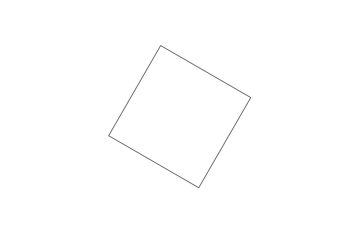

This is very handy… but probably also a bad idea! Because you have to post-multiply by the matrix, the sense of many affine transformations is reversed and construction of the matrix is not ‘by the book’. Usually the affine transformation matrix \(\mathbf{A}\) for an anti-clockwise rotation by angle \(\theta\) around the origin, would be

\[ \mathbf{A} = \left[\begin{array}{cc} \cos\theta & -\sin\theta \\ \sin\theta & \cos\theta \end{array}\right] \]

Here, because we are post-multiplying the rotation will be in the other direction… and to rotate anti-clockwise, you use the \(-\mathbf{A}=\mathbf{A}^T\)

\[ -\mathbf{A} = \left[\begin{array}{cc} -\cos\theta & \sin\theta \\ -\sin\theta & -\cos\theta \end{array}\right] = \left[\begin{array}{cc} \cos\theta & \sin\theta \\ -\sin\theta & \cos\theta \end{array}\right] = \mathbf{A}^\mathrm{T} \]

This means that if you are doing any serious affine transforming of sf shapes at a low-level in R spatial, I recommend either writing some wrapper functions that generate and apply the necessary matrices on the fly, or, probably better yet, using the wk package which has proper support for affine transformations.

Wrapper functions for the ‘native’ matrix operations

Taking the wk approach, I will show what you can do below. Making similar functions that just post-multiply shapes or add vectors to them instead is left as an exercise for the reader…

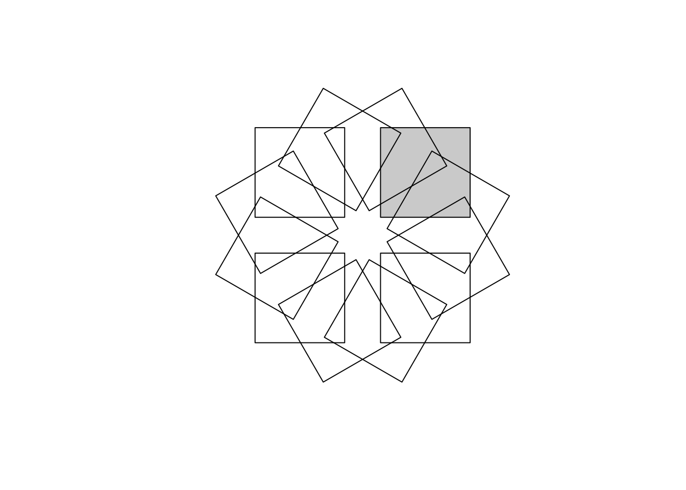
For example a rotation function might look something like

rotate_sf <- function(shp, angle) {
  wk::wk_transform(shp, wk::wk_affine_rotate(angle))
}

and this can be applied like this

base_s <- st_polygon(list(matrix(c(.25, 0.25, 
                                   1.5, 0.25, 
                                   1.5, 1.5, 
                                   .25, 1.5, 
                                   .25, .25), 
                                 nrow = 5, ncol = 2, byrow = TRUE)))
plot(base_s, xlim = c(-2, 2), ylim = c(-2, 2), 
     col = "lightgrey", border = NA)
for (a in seq(0, 330, 30)) {
  plot(rotate_sf(base_s, a), add = TRUE)
}

Or you might want to make multiple copies of a basic unit at a series of locations on a grid. First, make a function that will translate a shape by a vector.

translate_shape <- function(shape, translation) {
  wk::wk_transform(shape, wk::wk_affine_translate(translation[1], translation[2]))
}

Generate a set of translations

grid <- expand.grid(x = 0:19 * 1.2 + 1, y = 0:19 * 1.2 + 1)
squares <- list()
for (i in seq(nrow(grid))) {
  squares <- append(squares, 
                    list(translate_shape(square, c(grid$x[i], grid$y[i]))))
}
squares %>% sapply("[") %>% st_sfc() %>%
  plot()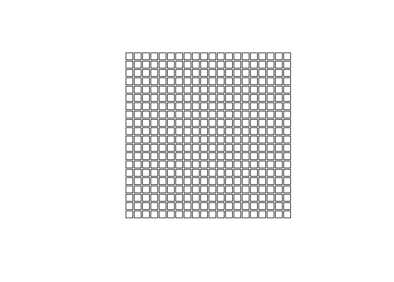

The wk functions also allow you to compose complex transformations from several steps. For example a function to rotate a shape around its own centre, i.e., not around the origin at \((0,0)\) requires moving the shape so that its centroid is at the origin, performing the rotation, then moving it back:

rotate_around_centroid <- function(shape, angle) {
  centroid <- st_centroid(shape) %>%
    st_coordinates() %>%
    c()
  transformation <- wk::wk_affine_compose(
    wk::wk_affine_translate(-centroid[1], -centroid[2]),
    wk::wk_affine_rotate(angle),
    wk::wk_affine_translate(centroid[1], centroid[2])
  )
  wk::wk_transform(shape, transformation)
}

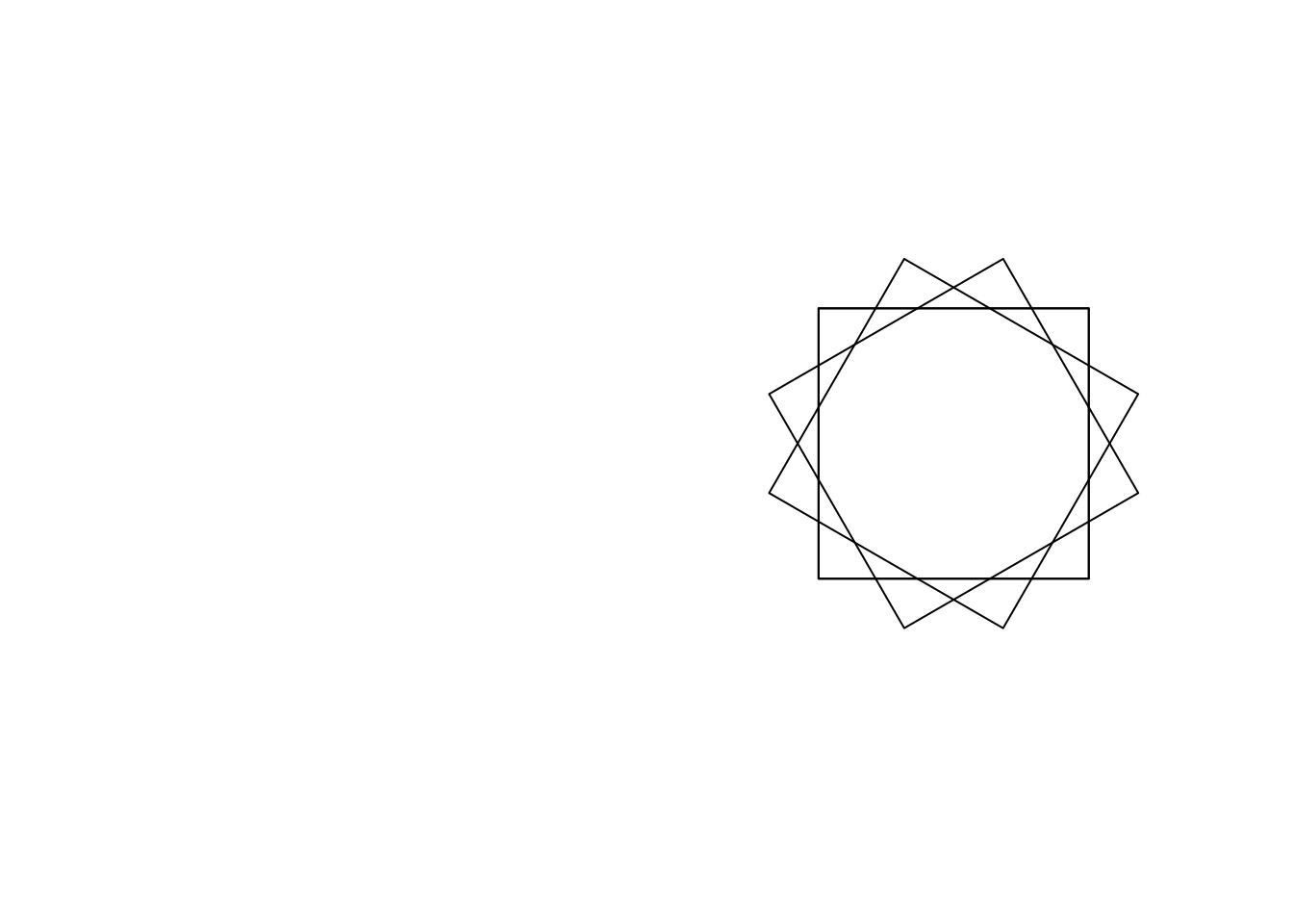
And here’s that in action

plot(square, xlim = c(-1, 1), ylim = c(-1, 1))
for (a in seq(30, 90, 30)) {
  plot(rotate_around_centroid(square, a), add = TRUE)
}