Into the (LiDAR) void

Last weekend the tables were turned on me by my elder son. Back when we lived in California, I dragged my two boys out on day hikes around the Bay Area much to their disgust (they had video games they’d rather have spent that time playing).

But lo and behold, a decade on and son #1 is planning on doing the :Te Araroa Trail next year sometime. Towards that end he’s doing a lot of overnight tramps and steadily working up to longer and more difficult expeditions (he’s done the :Tongariro Crossing and :Routeburn Track in the last couple of months, with another one coming up soon).

Anyway, back to his revenge. I haven’t done any serious tramping lately, but he took me on an overnight trip to the Waiopehu Hut in the :Tararua Range.

To cut a long story short and answer the question in my subtitle: I’m afraid of the Tararuas! OMG they’re gnarly. In all honesty, my son overestimated my abilities and although I made it in and back out, several days later I am still feeling it!

So where was this tramp?

Having admitted that I have a healthy respect for the Tararuas, I was disappointed to find in putting together this post, that they are a LiDAR deadzone for some reason. I’d hoped I could explore the fractal nature of our tramp from the comfort of my keyboard, but to do that well I’d need more precise elevation data than are available.

I’ve shown the LiDAR coverage available from LINZ overlaid on a LINZ Topo 50 map below. You can get the map data from here and of course there are also useful apps based on that layer. We also found the Organic Maps app which I have on my phone for everyday use, and which is based solely on OpenStreetMap data, to be very good.¹

topo_map <- rast("_data/nz-topo50.png")
crs(topo_map) <- st_crs(2193)$wkt
lidar_coverage <- st_read("_data/linz-lidar-available.gpkg")
path <- st_read("_data/path.gpkg") |> st_reverse()

tm_shape(topo_map) +
  tm_rgb() +
  tm_shape(lidar_coverage) +
  tm_fill(fill = "forestgreen", fill_alpha = 0.5) +
  tm_shape(path) +
  tm_lines(col = "black", lwd = 3) +
  tm_scalebar(position = tm_pos_out("center", "bottom"))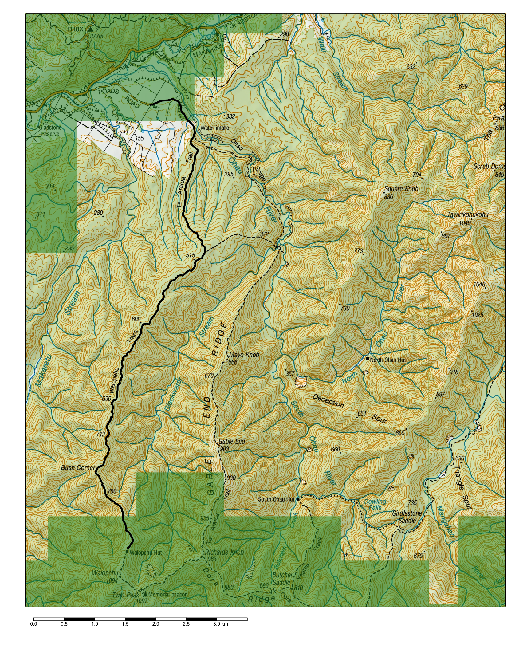

Without LiDAR data exploring the fractal nature of the ups and downs of the trail is a bit of a non-starter. The reason I wanted to look at it that way is that one of the most salient features of this track was just how much ‘down’ there is mixed in with the ‘up’. It’s a little bit ridiculous how much you end up resenting the downhill stretches on the way up, when you know you’re shortly going to have to pay for them with more uphill. Not only that, in terrain this rugged, going downhill might use less energy than going uphill, but it demands just as much concentration, if not more!

A transect of our travails

dem <- rast("_data/waiopehu-NZDEM_SoS_v1-0_14.tif")
hillshade <- rast("_data/hillshade.tif")
waterways <- st_read("_data/waterways.gpkg")

Anyway, here’s another map, assembled from data variously obtained from the Otago School of Surveying NZSoSDEMv1 15m digital elevation model and OpenStreetMap. I made the hillshade layer in QGIS. The School of Surveying DEM is the best available for ‘analysis’ purposes in this area that I’m aware of. LINZ offer an 8m product, but are careful to say it’s only useful for cartographic visualization. As it turned out, that’s all I ended up doing, but never mind, the 15m product is more than adequate for making a transect of the track.

tm_shape(dem) +
  tm_raster(col.scale = tm_scale_continuous(values = "hcl.terrain2")) +
  tm_shape(waterways) +
  tm_lines(col = "#89ddff",
           lwd = "waterway",
           lwd.scale = tm_scale_categorical(
             values = c(0.5, 1), levels = c("stream", "river"))) +
  tm_shape(hillshade) +
  tm_raster(col.scale = tm_scale_continuous(values = "-brewer.greys"),
            col_alpha = 0.15) +
  tm_shape(path) +
  tm_lines(col = "black", lwd = 3) +
  tm_layout(legend.show = FALSE)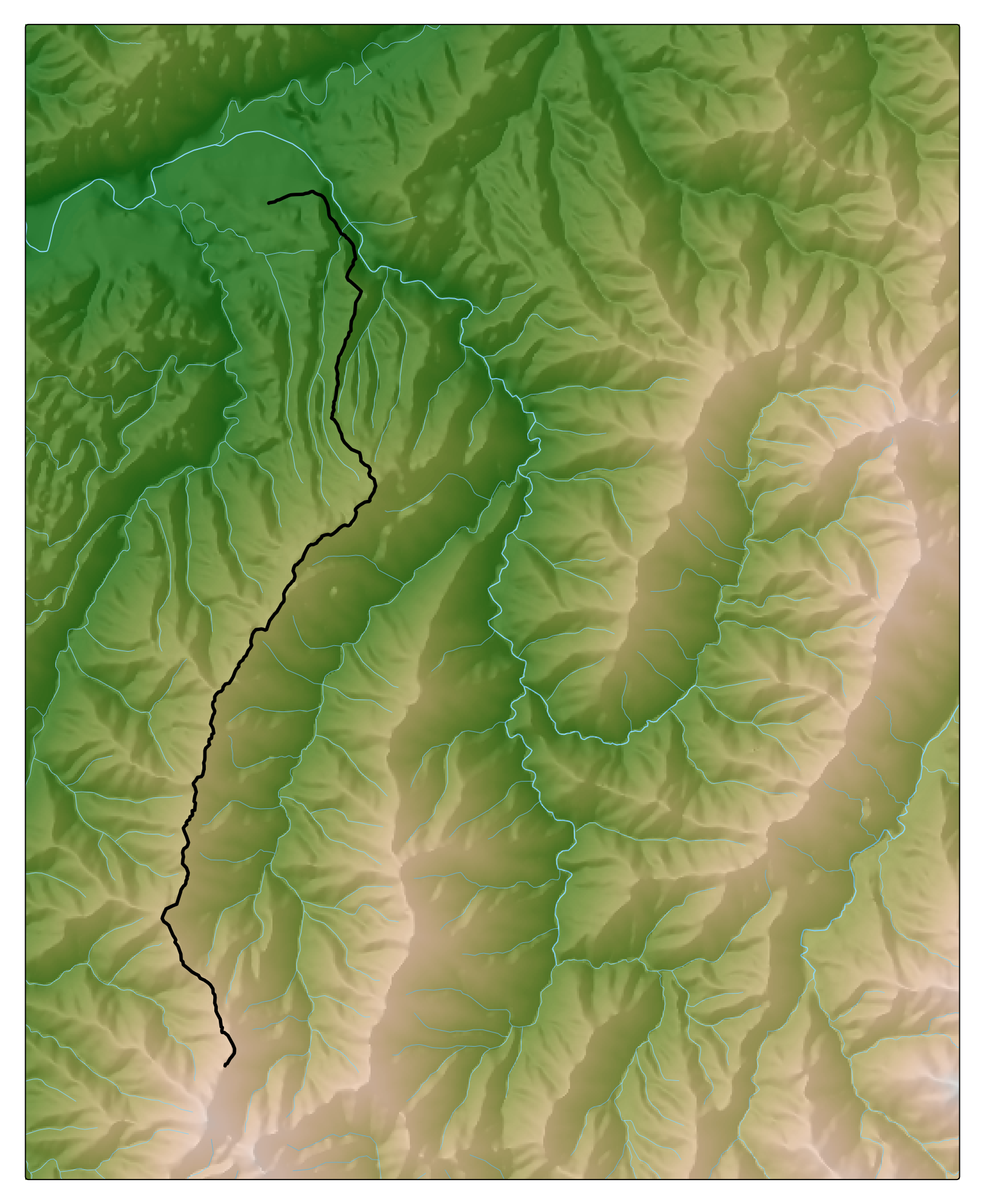

So here’s one approach to making a transect.

First we have to take the path, convert it to a series of points and extract elevation values from the DEM at those points. I’ve used just the points along the linestring rather than interpolating along its length. How that would look at different resolutions were LiDAR data available would be interesting to explore.

# function to return data for plotting a transect across a DEM along a line
get_transect <- function(dem, line) {
  pts <- line |> 
    st_cast("POINT") |>
    st_coordinates() |>
    as_tibble() |>
    st_as_sf(coords = 1:2, crs = st_crs(line))
  names(dem) <- "z"
  transect <- extract(dem, pts |> as("SpatVector"), 
                      method = "bilinear", xy = TRUE) |>
    as_tibble() |>
    mutate(dx = replace_na(x - lag(x), 0),
           dy = replace_na(y - lag(y), 0),
           dz = replace_na(z - lag(z), 0),
           dxy = sqrt(dx ^ 2 + dy ^ 2),
           distance = cumsum(dxy),
           Ascent = cumsum(if_else(dz > 0, dz, 0)),
           Descent = cumsum(if_else(dz < 0, dz, 0)),
           downhill_start = dz >= 0 & lead(dz) < 0,
           downhill_end = dz >= 0 & lag(dz) < 0) |>
    select(-dx, -dy, -dz, -dxy)
}

xyz <- dem |> get_transect(path)

1

First convert the LINESTRING to POINTs.

2

Extract the point coordinates.

3

Convert back to an sf dataset.

4

Make sure the height variable in the DEM is called z.

5

The terra::extract function extracts values from the DEM at the supplied points (which have to be converted to a SpatVector layer for this to work). xy = TRUE ensures that the x, y coordinates are also retained in the output.

6

The lag function allows us to calculate differences between consecutive values in the data frame. The first difference will come out as a NA result (since there is no value before the first row), so we use replace_na to set that result to 0.

7

Use cumsum to calculate a elapsed distance from the start, and also total ascent and descent determined separately.

8

Detecting when downhill sections of the trail start and end.

For plotting purposes it’s easier if we pull the data apart into two data frames, one with the cumulative ascent and descent data tagged as such, the other with them retained, and with a constant label added. This is mostly so that we can convince ggplot to give us two items in the plot legend!

up_down <- xyz |> 
  select(distance, Ascent, Descent) |>
  pivot_longer(cols = c(Ascent, Descent))

transect <- xyz |>
  select(distance, Ascent, Descent) |>
  mutate(height = Ascent + Descent,
         gain = as.factor(c("Gain")))

1

Because descent values are negative we just add Ascent and Descent to get the net climb.

2

The gain variable is constant, but used here so that it can be picked up by scale_colour_manual which persuades ggplot to produce a legend item for it.

Finally we can make a plot.

g <- ggplot() + 
  geom_area(
    data = up_down, 
    aes(x = distance, y = value, group = name, fill = name),
        colour = NA, position = "identity", alpha = 0.35) +
  scale_fill_brewer(palette = "Set1", name = "Up or down") +
  geom_line(
    data = transect, 
    aes(x = distance, y = height, colour = gain)) +
  scale_colour_manual(name = "", values = "black", labels = "Net gain") +
  coord_cartesian(expand = FALSE) + 
  labs(x = "Elapsed distance, m", y = "Height gain from start, m")

g + theme_minimal()

I have split the climb out like this, because as I said above, some of the more emotionally uh… challenging parts of this trip were the sections going downhill when our overall course was up, and I wanted to see just how much of that there was.

It looks like a pretty relentless uphill tramp. But there really are quite a few sections of downhill. To emphasise this we can add to the plot, using the downhill start and end flags in the data.

downhill_starts <- xyz |>
  filter(downhill_start) |>
  pull(distance)

downhill_ends <- xyz |>
  filter(downhill_end) |>
  pull(distance)

downhill_sections <- tibble(
  dmin = downhill_starts,
  dmax = downhill_ends)

g + geom_rect(data = downhill_sections, 
              aes(xmin = dmin, xmax = dmax, 
                  ymin = min(xyz$Descent), 
                  ymax = max(xyz$Ascent)),
              fill = "#00000030") +
  theme_minimal()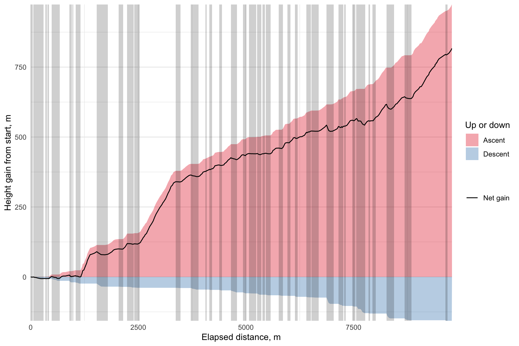

And now we can see that while many of those ‘downhill’ sections on the way up are really fairly level, there are a lot of them!

All in all, I’m not sure I’d recommend it as a first long hike back after a (too) long break. Maybe I’ll go back next year and see if I’ve gotten any fitter.

Meanwhile, here’s a photograph looking further to the east from the hut when we finally got there. Lighting conditions were a bit challenging for my phone’s camera, but all in all… very much worth it, even if I won’t be hurrying back right away!

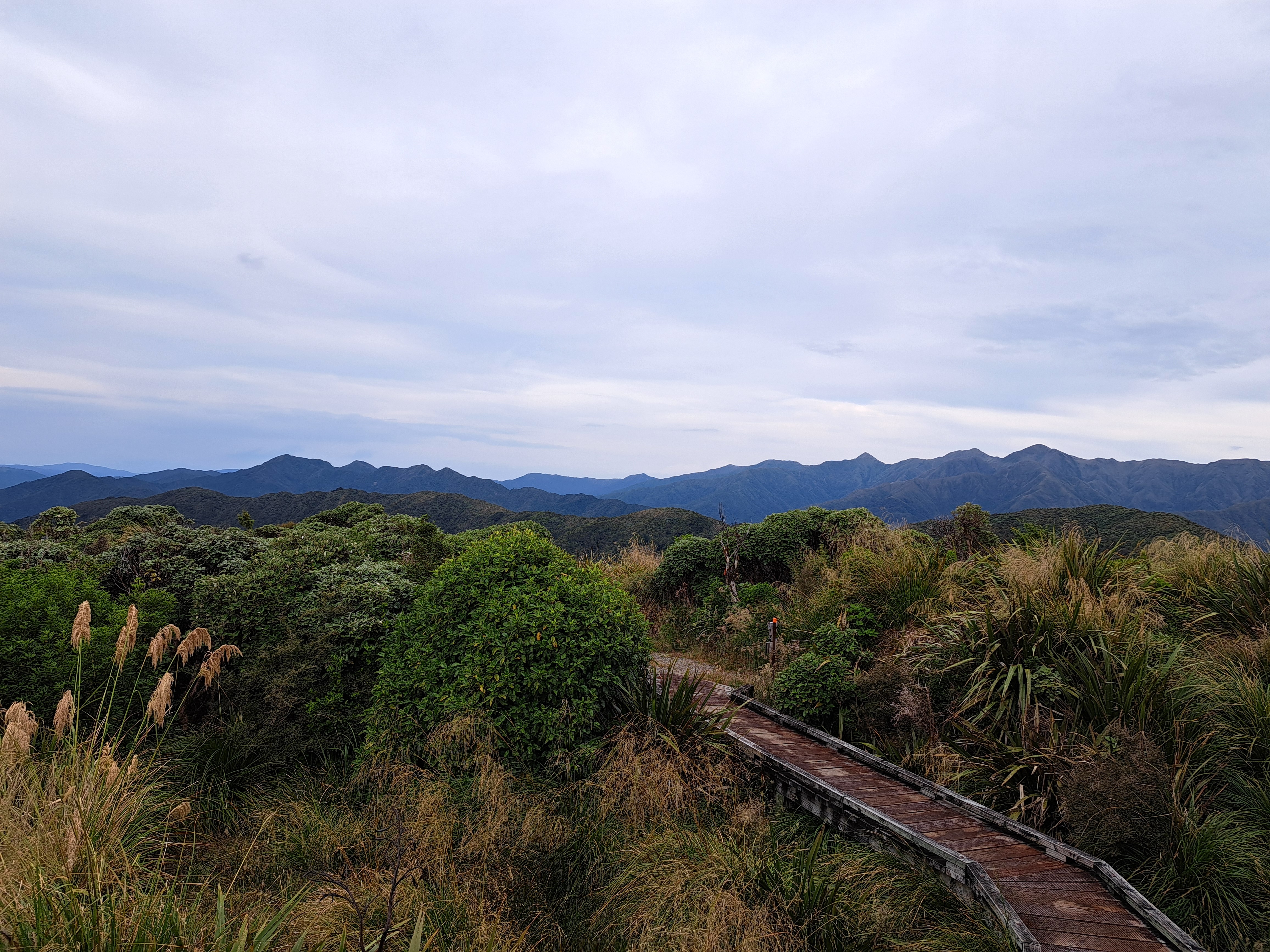
Footnotes

1. But take my advice: don’t take my advice on anything to do with tramping.