An attempt to rank the nine examples of so-called ‘bad map projections’ published by the XKCD web comic over the last few years. Not all the projections are actually bad, and I managed to reproduce some in R.
geospatial
R
tutorial
stuff
cartography
xkcd
Author
David O’Sullivan
Published
May 16, 2025
Warning: sensitive souls who care about geodetic accuracy should probably stop reading now. Liberal use of affine transformation of geometries throughout. You have been warned.
For a long time I thought about teaching a geography / GIS class using XKCD comics as the primary source material, or at the very least as a jumping off point for every lecture. Recently I actually went through every XKCD from the very beginning to the present to assemble a list of comics that would actually be usable in some semi-serious2 way for this purpose. Among the things I learned is that Randall Munroe has become a lot less fixated on sex than he was when he started, and also somewhat less worried about velociraptors.
Also, his interest in map projections only seems to have kicked in about halfway through the XKCD time series. Possibly this is related to an ongoing interest in GPS, which will likely be a topic for a future post. #977 Map projections posted in late 2011, is the first sign of an enduring interest in projections, but things don’t really take off until #1500 almost 4 years later, which is the first of several ‘bad map projections’, although not actually called out as such in its title.
Herewith, my ranking from worst bad projection to best bad projection of the nine examples I found,3 accompanied in a few cases by attempts at recreating them in R (click on the code-fold links to see how). Eventually, perhaps, ongoing work on arbitrary map projections might enable me to automate reverse-engineering any XKCD projection. For now, a combination of perseverance, guess-work, and sheer bloody mindedness will have to suffice.
For forming proj strings that include values from data.
4
To densify some shapes.
5
The less said about this the better.
For what it’s worth, by worst bad projection I mean something like ‘least interesting’ and by best, I mean something like ‘most thought-provoking’.4
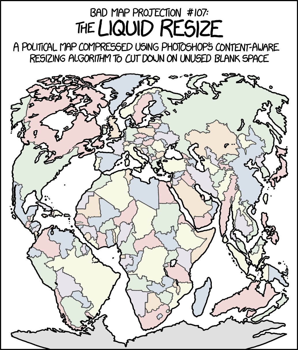
#9 Bad Map Projection: Liquid Resize
Alt-text: This map preserves the shapes of Tissot’s indicatrices pretty well, as long as you draw them in before running the resize.
I don’t use Adobe Photoshop so XKCD 1784 is just a bit too inside baseball for me. It feels like there might be a missed opportunity here to have said something about continental drift and Pangaea and supercontinents, which is a topic that has come up in other XKCDs (see # 1449 Red Rover). Something about how Africa and South America fitting together so well is evidence for plate tectonics liquid resize.
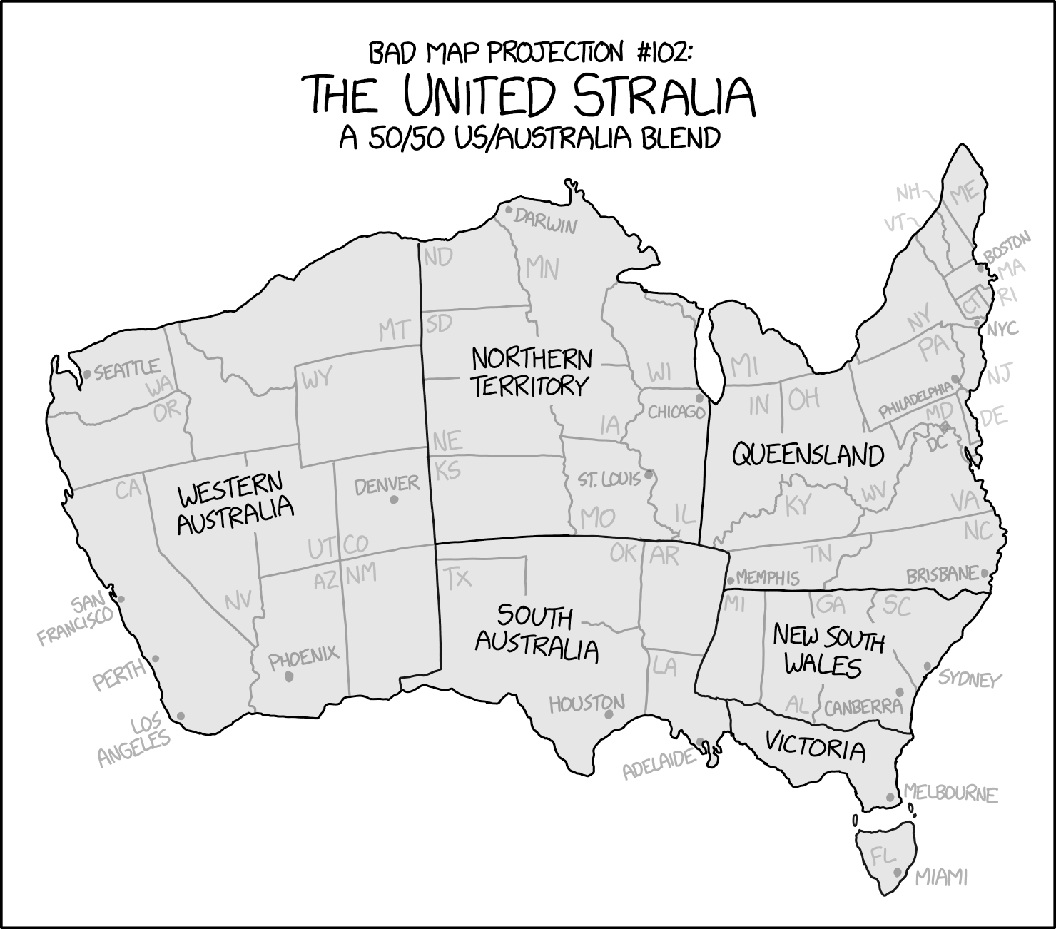
#8 Bad Map Projection: The United Stralia
Alt-text: This projection distorts both area and direction, but preserves Melbourne.
XKCD 2999 just doesn’t work for me.5 I appreciate the attempt at many to one projection, that is to say more than one place on Earth mapping onto a single location in the map. And it’s certainly a relief to know that Melbourne is preserved.6
I didn’t even try to replicate this one as it seems self-evidently something you’d have to do in a drawing package. Overall, I think the idea of two places into one is much better realised elsewhere in this list.
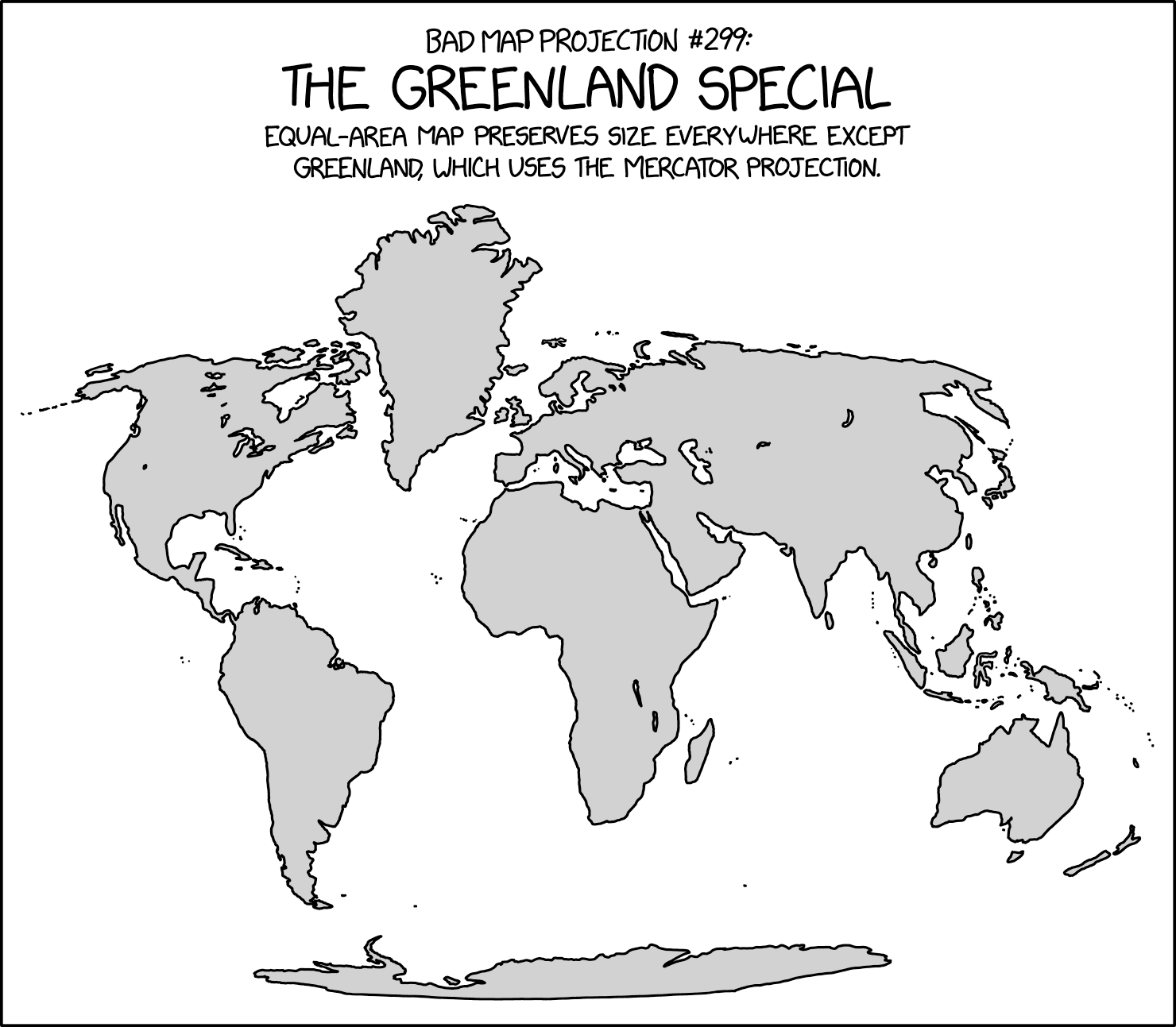
#7 Bad Map Projection: The Greenland Special
Alt-text: The projection for those who think the Mercator projection gives people a distorted idea of how big Greenland is, but a very accurate idea of how big it SHOULD be.
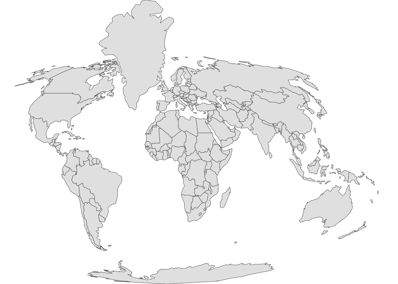
The whole Greenland thing in map projections is a bit played out. I realise it continues to blow minds how exaggerated its size is in the Mercator projection.7 Anyway, it’s not too hard to remake XKCD 2489 using R, provided you aren’t too respectful of, you know, actual projections. Apparently Mercator Greenland is too big even for this comedy projection, as I had to downscale it to 85% of its ‘raw’ Mercator size to get a good match to the published map.
Experimentation suggested that some rescaling of Greenland as it is projected ‘raw’ is required to get the outcome in the comic.
2
After rescaling and shifting Greenland we have to tell a white lie and tell R the data are still Mercator projected.
3
A buffered Greenland clears a passage between Greenland and Canada.
4
Fairly confident the rest of the world is Mollweide projected.
5
It’s not uncommon for world data sets to have invalid polygons after projection and that’s the case here.
6
This erases the existing Greenland and removes some of Canada’s offshore islands.
7
Add Mercator Greenland into the data.
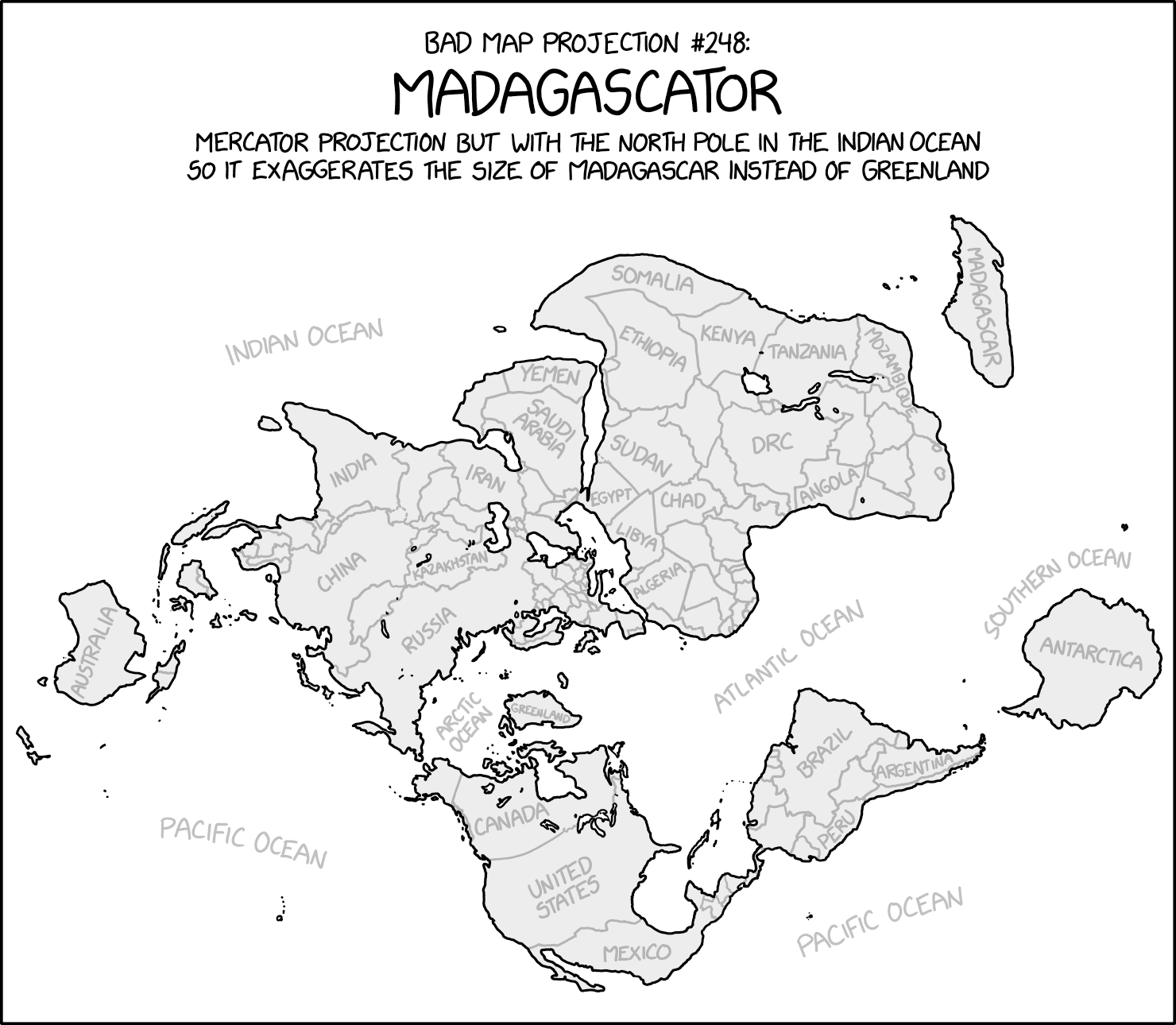
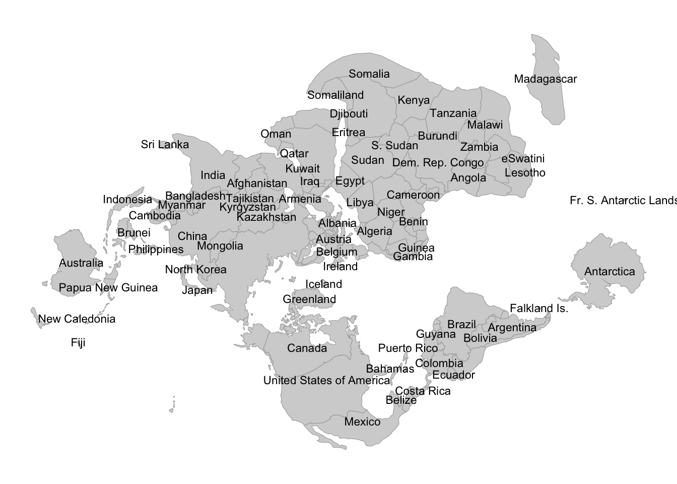
#6 Bad Map Projection: Madagascator
Alt-text: The projection’s north pole is in a small lake on the island of Mahé in the Seychelles, which is off the top of the map and larger than the rest of the Earth’s land area combined.
XKCD 2613 went up in my estimation after I figured out how to make it… the alt-text provides enough information to find the central coordinates, which are in La Gogue Lake on Mahé in the Seychelles.
Armed with the ludicrously precise lat-lon coordinates8 Google provided me for this spot, I figured out how to approximate this map.
Those ludicrously precise coordinates from Google.
2
Tell sf that the data are centred on somewhere different than they really are! Some experimentation was required here to find a central ‘meridian’ that didn’t cut Antarctica in half.
3
Apply Mercator to the recentred data. There’s probably a setting of the Oblique Mercator (+proj=omerc) that can do this sequence of transforms in one go, but since what I have works, I am leaving well alone.
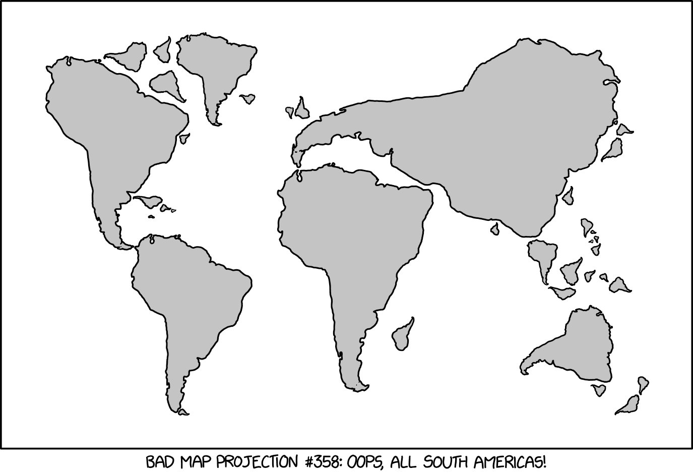
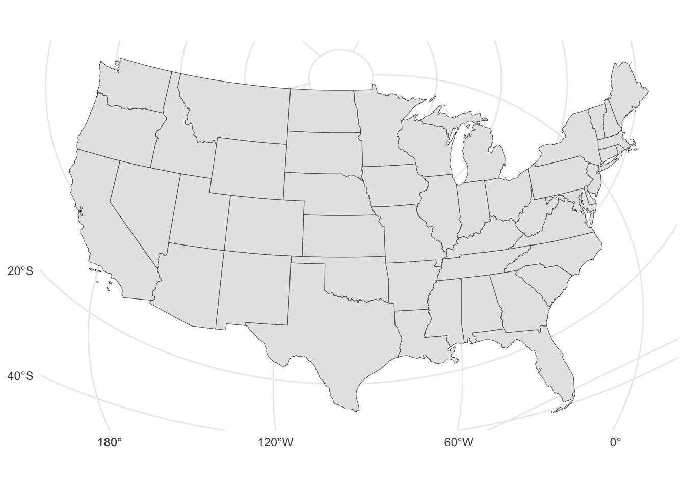
#5 Bad Map Projection: South America
Alt-text: The projection does a good job preserving both distance and azimuth, at the cost of really exaggerating how many South Americas there are.
XKCD 2256 is just delightfully dumb really. Truly a bad map projection. It’s also hard (for me) not to love a map projection that will throw everyone doing Worldle off their game.
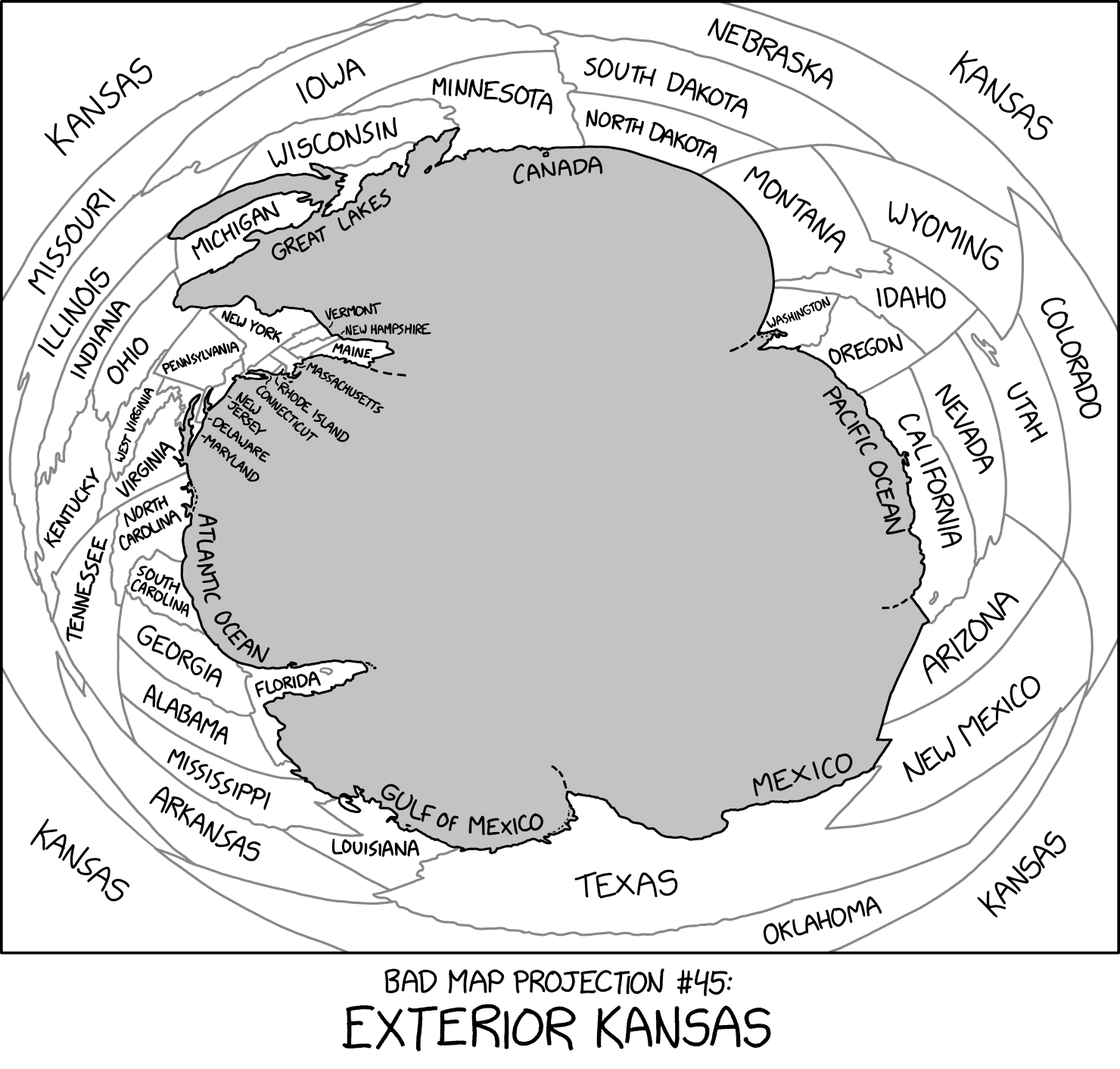
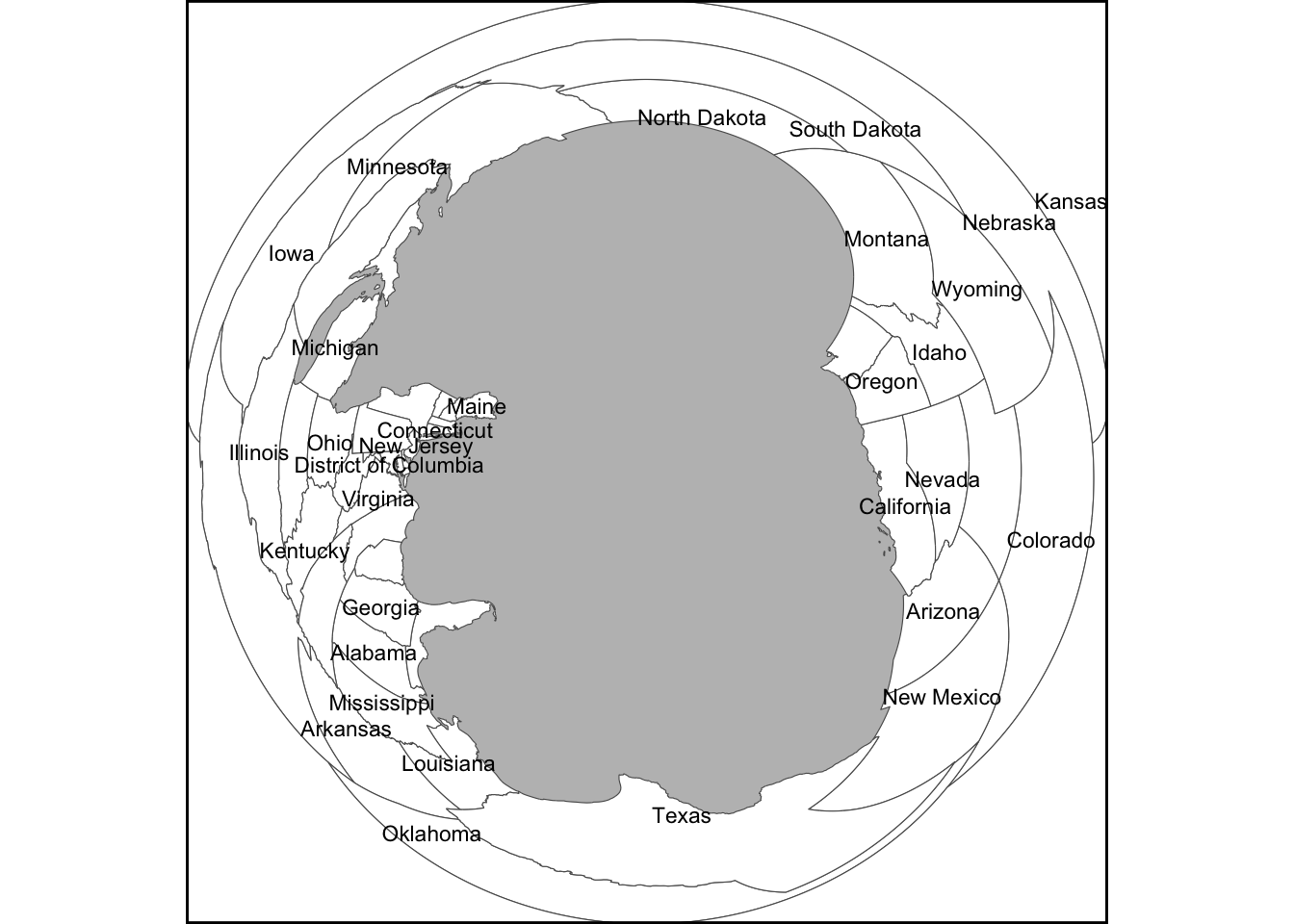
#4 Bad Map Projection: Exterior Kansas
Alt-text: Although Kansas is widely thought to contain the geographic center of the contiguous 48 states, topologists now believe that it’s actually their outer edge.
The ‘comical’ claim about topologists in the alt-text for XKCD 2951 is actually… well… true on a spherical surface.
I figured out a way to approximate this projection. First, we project the contiguous 48 states centred on the geographic center and enlarge them so they ostensibly cover a greater part of Earth’s surface. Any projection should work here; I’ve used an azimuthal equidistant one.
Forward projection: this can likely be any sensible projection with a central coordinate pair.
4
The distance projection from the antipode, that will ‘invert’ the space.
5
This multiplication expands the extent of the states.
6
After the multiplication we have to reset the projection.
Next we apply an azimuthal equidistant projection centred on the antipode of the geographical centre. At this point we have to ‘turn Kansas inside out’, then remove and add it back into the inverted states.
Make ‘inverse’ Kansas by subtracting Kansas from the bounding box of the data.
2
Remove Kansas.
3
Add back inverted Kansas.
And now we can make the final map. Note that it seems like an adjustment to the aspect ratio has been applied in the comic. I’ve not bothered with that step here. I assume that at some point Randall Munroe exports map data to a drawing package and does final tweaks there.
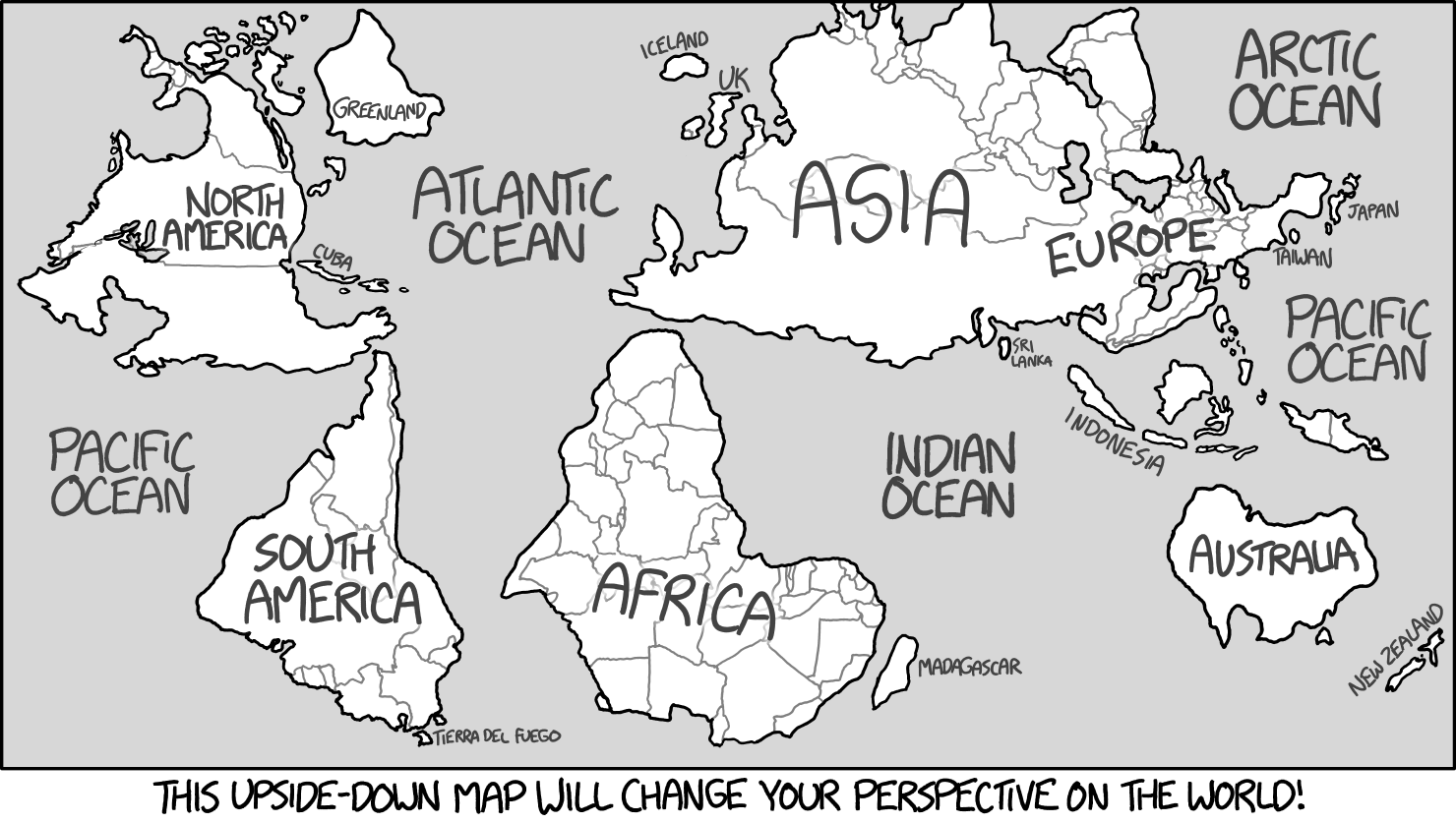
Alt-text: Due to their proximity across the channel, there’s long been tension between North Korea and the United Kingdom of Great Britain and Southern Ireland.
Personally, living in Aotearoa New Zealand I enjoy the genre of ‘upside down’ maps, but have always felt that the notion they change your whole perspective on the world is overstated, so XKCD 1500 is a nice gentle undermining of that, which I appreciate.9
I briefly contemplated an attempt at making this one, but thought better of it. Turning a whole map through 180° is not difficult:
Likely the easiest way to make this into a map like the one in the comic is to export to a drawing format and move things around by hand.
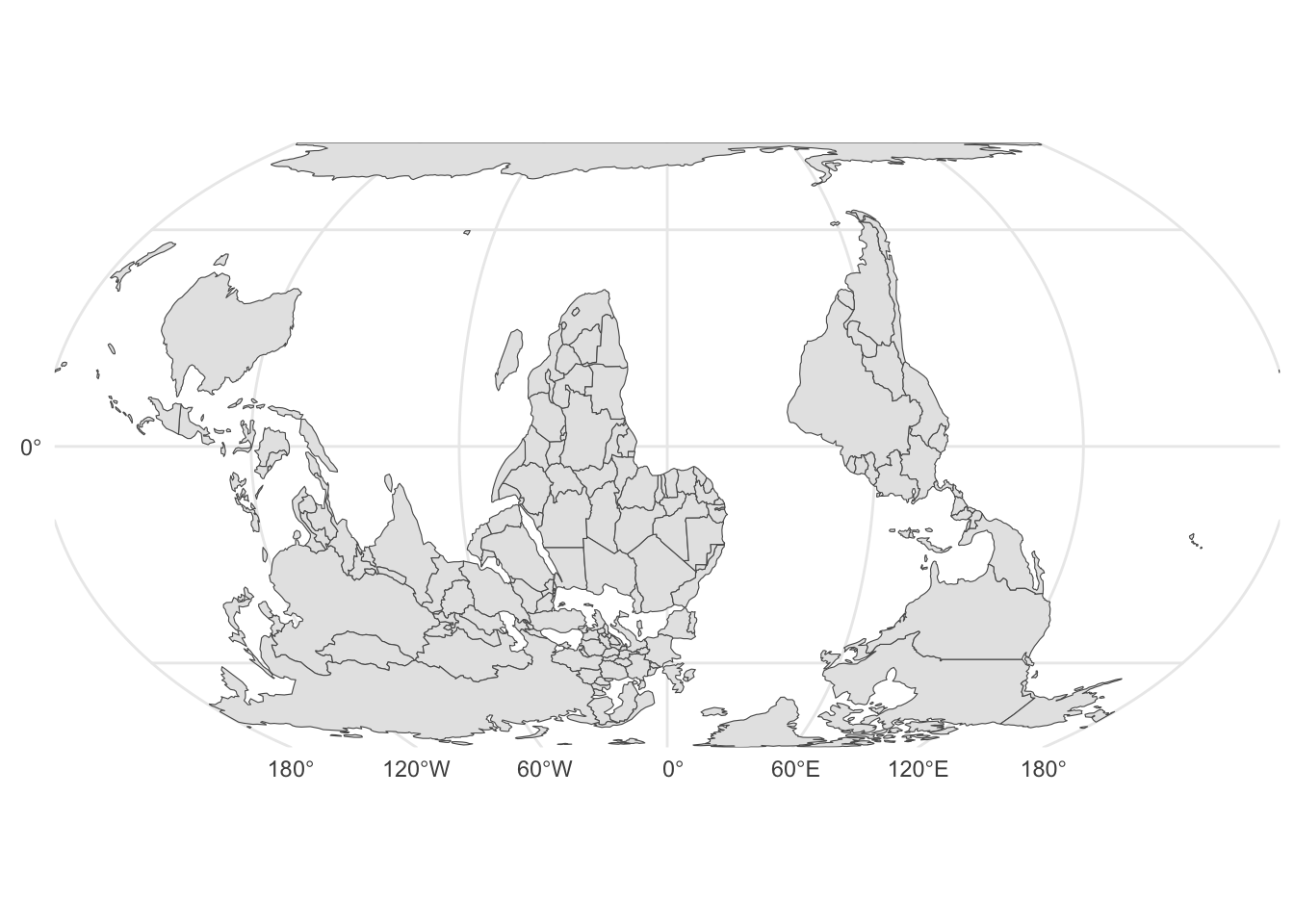
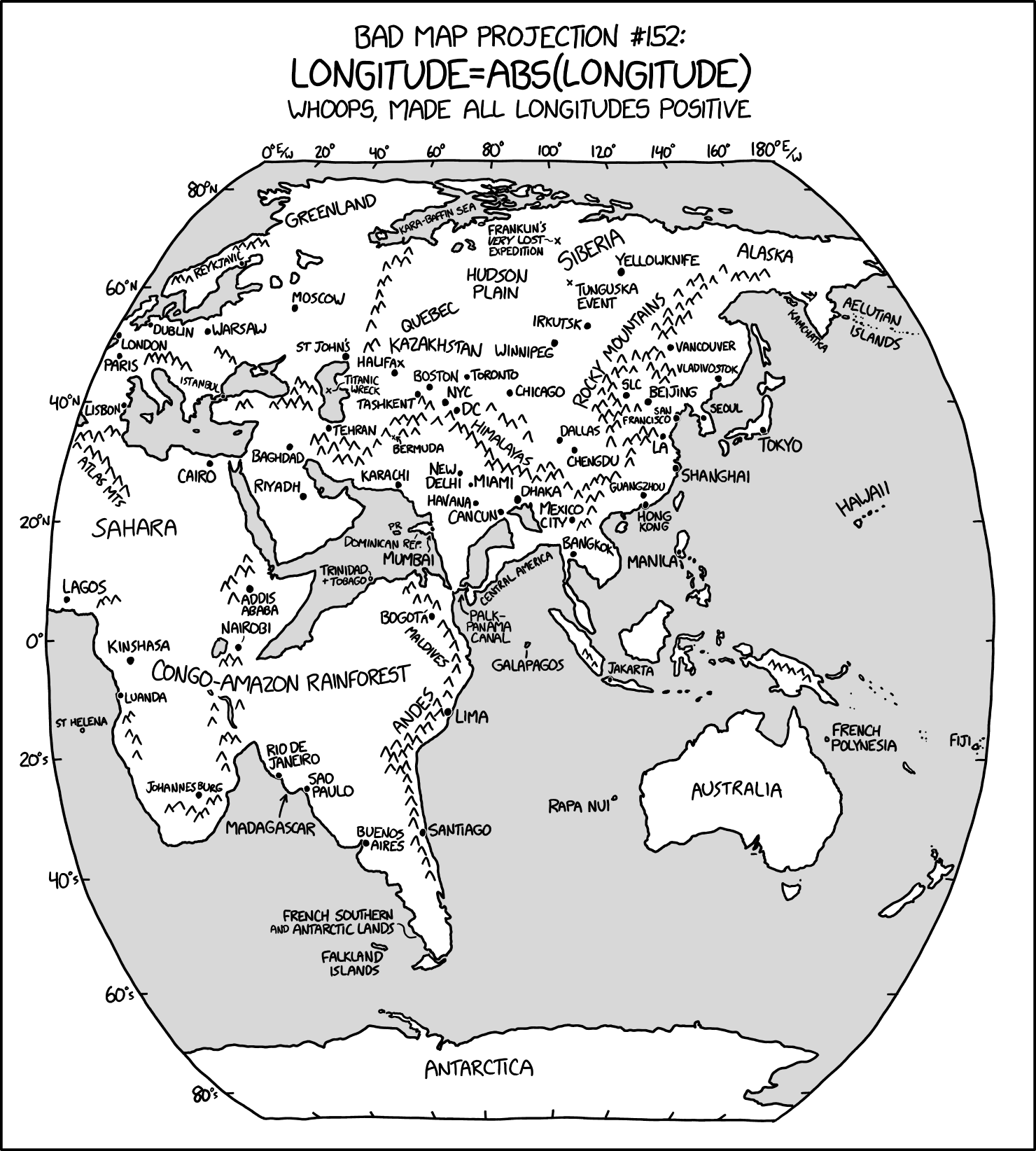
#2 Bad Map Projection: ABS(Longitude)
Alt-text: Positive vibes/longitudes only
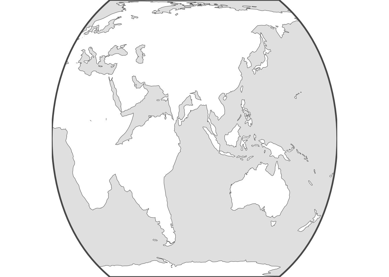
If only rendering XKCD 2807 was as easy as doing longitude = abs(longitude).10 In R things get a bit more involved. This would really be very straightforward in a drawing package.
It’s convenient to have a function for making hemispheres centred on a specified meridian.
2
The density parameter gives us hemispheres that still look right after transformation to a non-rectangular projection.
3
An educated guess that the map is in the Equal Earth projection.
4
This is where we make all longitudes positive.
5
Combine the hemispheres and shift them so they are centred on the prime meridian and transform to Equal Earth
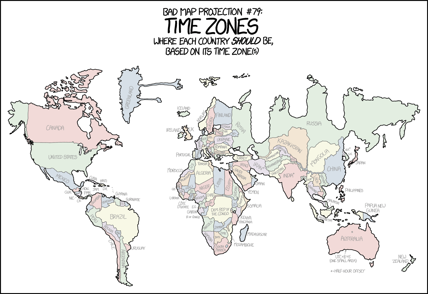
#1 Bad Map Projection: Time Zones
Alt-text: This is probably the first projection in cartographic history that can be criticized for its disproportionate focus on Finland, Mongolia, and the Democratic Republic of the Congo.
I’m really not convinced XKCD 1799 is a bad map projection. It looks wonky as hell, but it’s certainly useful, which is all we can ask of any projection.11 I’m fairly confident Waldo Tobler would have approved, although I never had an opportunity to ask.
It’s interesting to contemplate what kind of automated process might be used to produce this map, but… I’m not even going to try. Happy to hear from anyone who gives it a go!
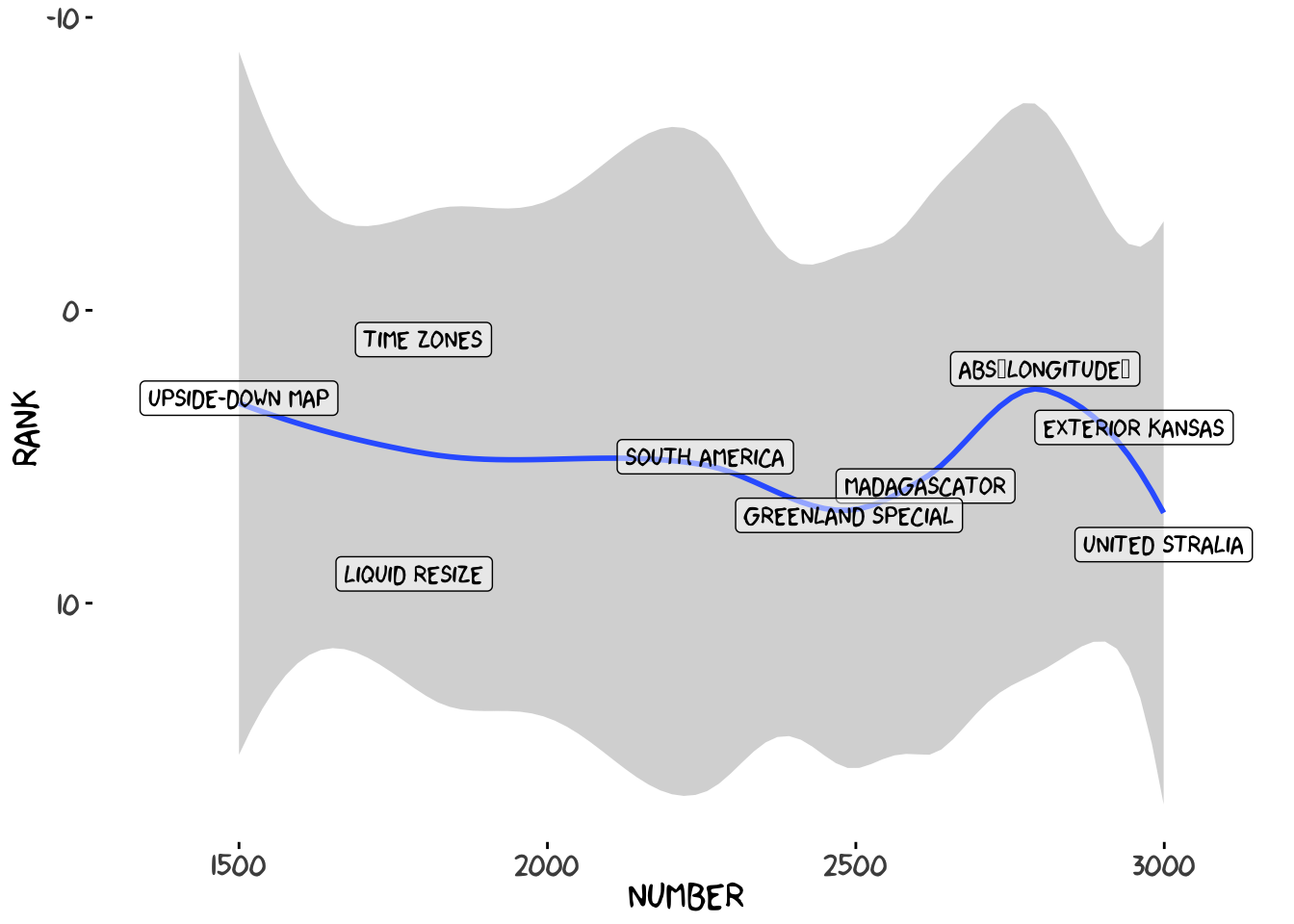
In conclusion
Close analysis of the data confirms no clear long term trend in the badness of XKCD’s bad map projections, although more recent examples may be getting worse.12
And that’s a wrap (or fold, or cut, or… some transformation anyway).
Footnotes
Insert ‘You won’t believe how bad they are’ or similar clickbait headline here.↩︎
We’re working with a loose definition of the word ‘serious’ here.↩︎
Along with #1500 which was not called out as such↩︎