Code
library(sf)
library(units)
library(dplyr)
library(tidyr)
library(ggplot2)
library(patchwork)

nz <- st_read("nz-islands.gpkg")Rather obviously, the proper names for Aotearoa New Zealand’s two largest islands are Te Ika-a-Maui and Te Waipounamu. It’s not just that those are the names given by the indigenous peoples of the whenua (and also official names), it’s that the extremely boring ‘North Island’ and ‘South Island’ are wrong. Or at any rate, not entirely right.
That’s a bold claim. Let me explain with the help of some uh… in-depth spatial analyis.
library(sf)
library(units)
library(dplyr)
library(tidyr)
library(ggplot2)
library(patchwork)
nz <- st_read("nz-islands.gpkg")So here’s a usefully labelled map of the three big islands along with quite a few smaller offshore islands.1
ggplot(nz) +
  geom_sf(aes(fill = north), lwd = 0) +
  scale_fill_brewer(palette = "Set1", direction = -1) +
  theme_void()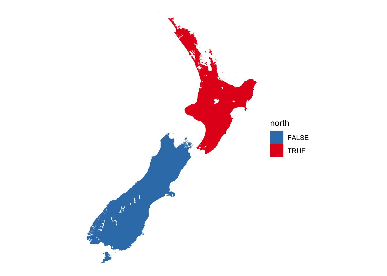
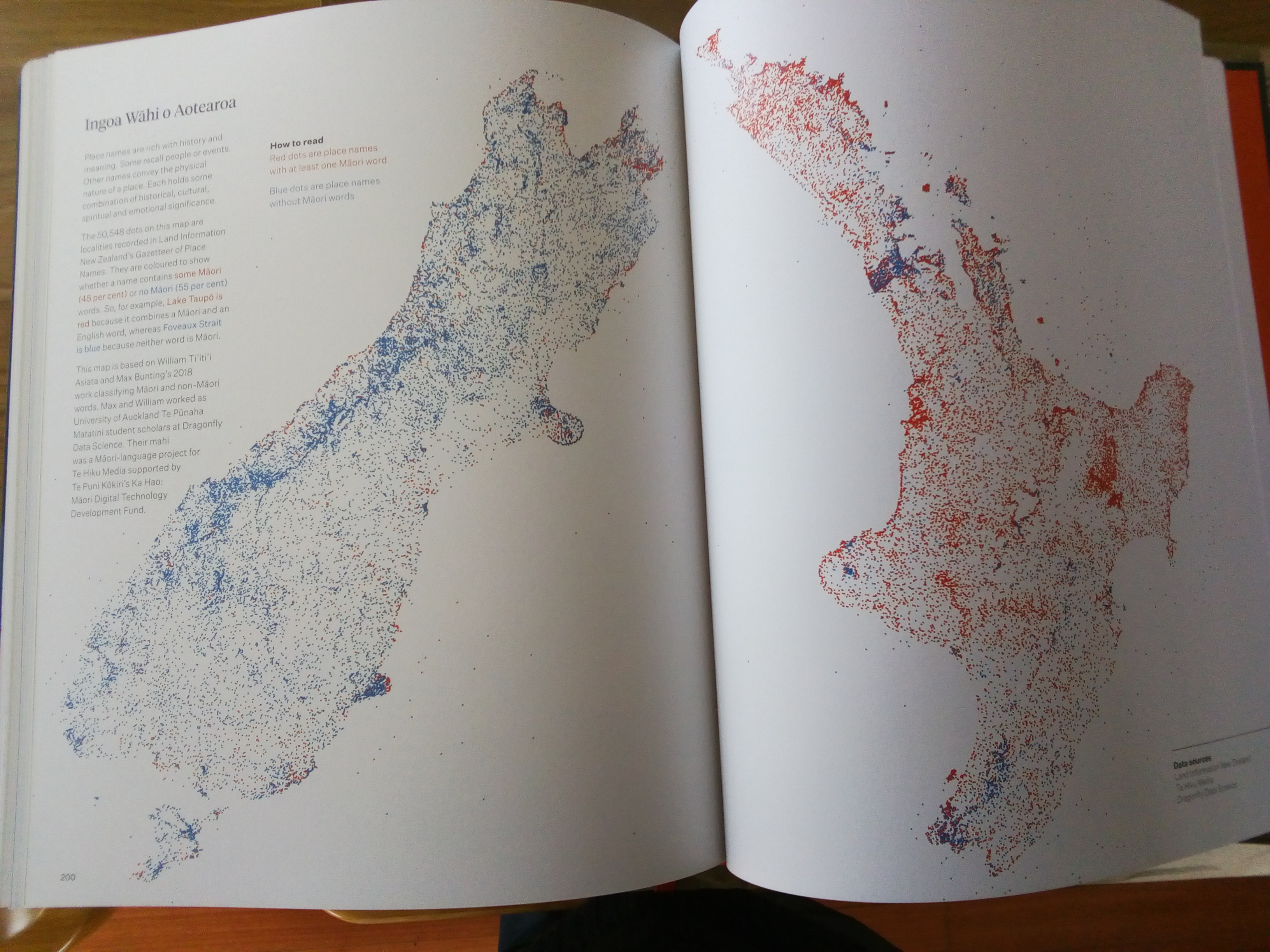
I considered colouring Te Ika-a-Māui blue and Te Waipounamu red, for the respective colours of their allegedly strongest sports teams. But I’m not much invested in rugby, and Wellington are clearly the best cricket team,2 so I’ve inverted what many might consider the ‘natural’ colours for the two islands. This is also a nice echo of one of my favourite spreads from Chris McDowall and Tim Denee’s wonderful We Are Here:
Anyway, if you look at that north-south map, it’s not entirely clear that east-west isn’t just as accurate a binary. If we randomly sample the islands, we get a sense of how strongly aligned north/east and south/west designations are.
pts <- nz |>
  st_sample(1000) |>
  st_coordinates() |>
  as.data.frame()

ggplot(nz) +
  geom_sf(lwd = 0) +
  geom_point(data = pts, aes(x = X, y = Y), size = 0.25) +
  geom_smooth(data = pts, aes(x = X, y = Y), method = "lm") +
  coord_sf(datum = 2193) +
  theme_minimal()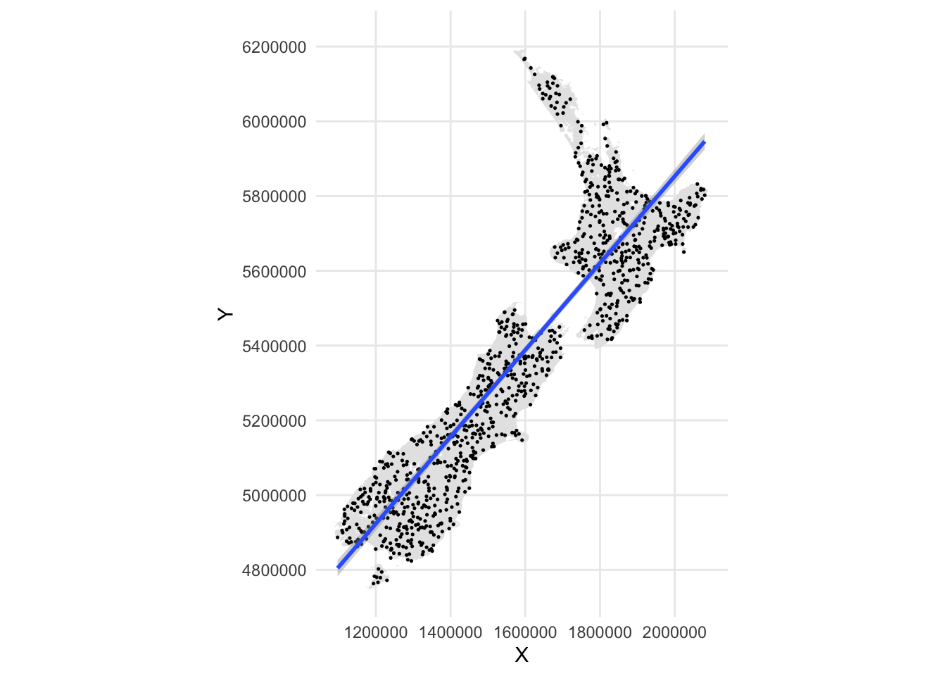
We can even put a number on this observation.
cor(pts) X Y
X 1.0000000 0.8515348
Y 0.8515348 1.0000000With pretty high accuracy, if a place is in the ‘north’, it is in the ‘east’! There are probably better ways to ‘put a number’ on this observation (contingency tables and whatnot), but a correlation coefficient will do for now.
To be serious—for just a paragraph—this correlation between latitudes and longitudes is something to be aware of when doing spatial modelling. In the context, for example, of species distribution models, it’s an open question if latitude or ‘island’ is a better variate to include for this reason, and it’s certainly questionable due to collinearity to include both latitude and longitude in models.3
To put areas on this perspective, we can slice the islands at their mutual centroid. First get a bounding box, and a centroid.
bb <- nz |> st_bbox()
centroid <- nz |>
  st_union() |>
  st_centroid() |>
  st_coordinates() |>
  c()
Next make a function to move one bound of a bounding box and turn it into a simple features data set.
bbox_split <- function(bb, ctr, half = "N") {
key <- c(N = "ymin", S = "ymax",
E = "xmin", W = "xmax")
coord <- c(N = 2, S = 2, E = 1, W = 1)
bb |> replace(key[half], ctr[coord[half]]) |>
st_as_sfc() |>
as.data.frame() |>
st_sf()
}And now we can split the country in each of these two directions.
ns_split <- bind_rows(
bbox_split(bb, centroid, "N") |> mutate(north_c = TRUE),
bbox_split(bb, centroid, "S") |> mutate(north_c = FALSE))
ew_split <- bind_rows(
bbox_split(bb, centroid, "E") |> mutate(east_c = TRUE),
bbox_split(bb, centroid, "W") |> mutate(east_c = FALSE))
nz_split <- nz |>
st_intersection(ns_split) |>
st_intersection(ew_split) |>
mutate(ns_correct = north_c == north,
ew_correct = east_c == north) |>
group_by(ns_correct, ew_correct) |>
summarise() |>
mutate(area = st_area(geom) |> set_units("km^2"))group_by |> summarise makes for nicer maps.
And we get the calculated areas below.
nz_split |> st_drop_geometry()# A tibble: 4 × 3
# Groups: ns_correct [2]
ns_correct ew_correct area
* <lgl> <lgl> [km^2]
1 FALSE FALSE 7169.
2 FALSE TRUE 7334.
3 TRUE FALSE 11494.
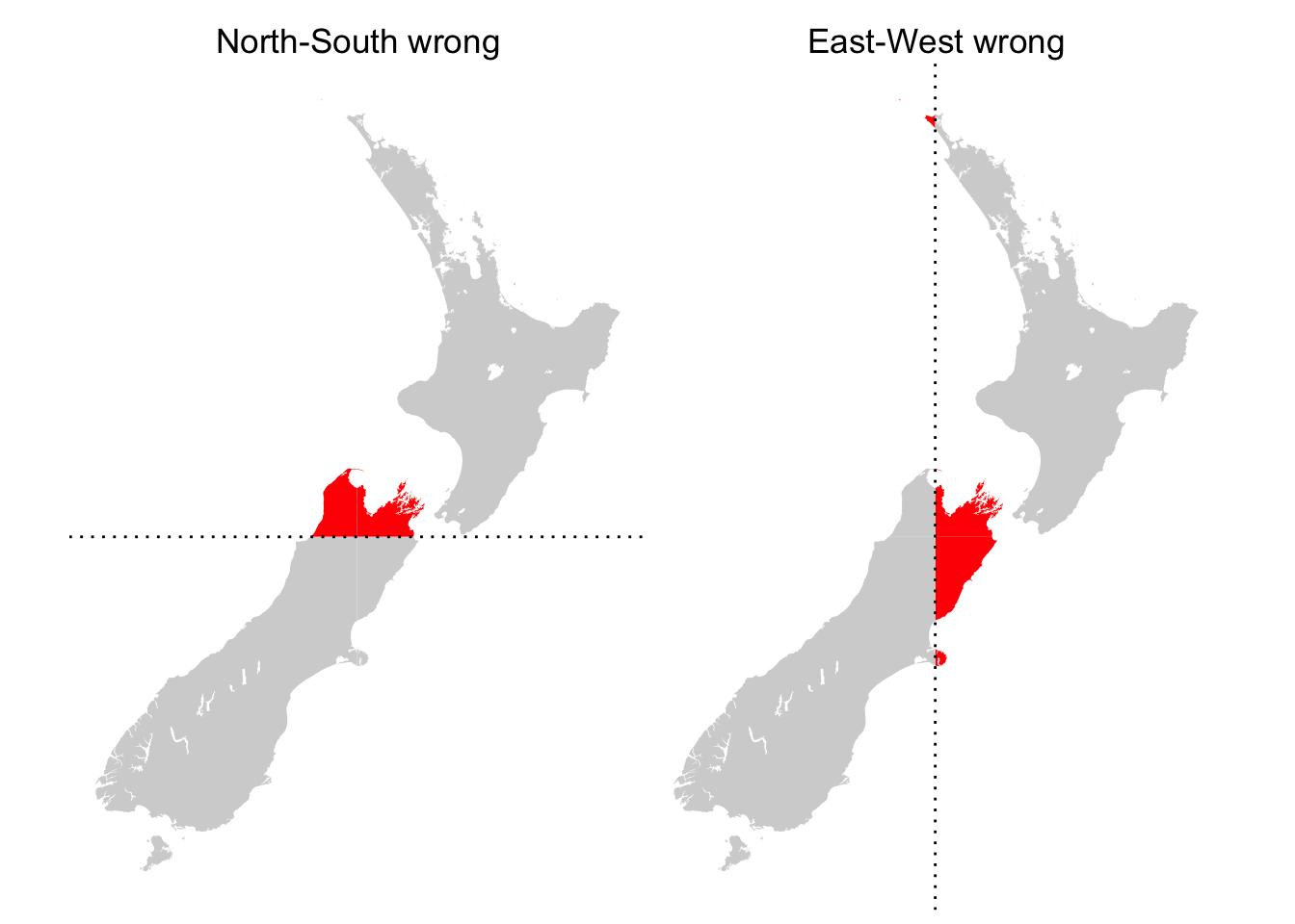
4 TRUE TRUE 238720.To my (slight) disappointment north-south is less wrong than east-west would be, although not by much. Oh well, so much for that idea.
Here are a couple of maps in case you’re missing them in that blizzard of code. Notably the very tip of Te Ika-a-Māui winds up in a notional ‘west’ island, and to the distress of many, a chunk of Canterbury winds up lumped with the ‘east’ island.4
map1 <- ggplot(nz_split) +
geom_sf(aes(fill = ns_correct), lwd = 0) +
scale_fill_manual(breaks = as.logical(0:1),
values = c("red", "lightgrey")) +
geom_hline(aes(yintercept = centroid[2]), linetype = "dotted") +
guides(fill = "none") +
ggtitle('North-South wrong') +
theme_void() +
theme(plot.title = element_text(hjust = 0.5))
map2 <- ggplot(nz_split) +
geom_sf(aes(fill = ew_correct), lwd = 0) +
scale_fill_manual(breaks = as.logical(0:1),
values = c("red", "lightgrey")) +
geom_vline(aes(xintercept = centroid[1]), linetype = "dotted") +
guides(fill = "none") +
ggtitle('East-West wrong') +
theme_void() +
theme(plot.title = element_text(hjust = 0.5))
map1 + map2patchwork package here rather than facetted plots.
At this point, I contemplated finding a decision boundary for points sampled from the islands, but I haven’t (yet) lost it completely.5
A more rough and ready approach involved jiggling geom_abline around a bit until it threaded through the Cook Strait / Te Moana-o-Raukawa.
hulls <- nz |>
  group_by(north) |>
  summarise() |>
  st_convex_hull()

g1 <- ggplot(nz) +
  geom_sf(lwd = 0) +
  geom_sf(data = hulls, fill = NA, colour = "red") +
  geom_abline(aes(intercept = 9.6125e6, slope = -2.414214),
              linetype = "dashed") +
  annotate("polygon", x = c(1.65e6, 1.65e6, 1.75e6, 1.75e6),
                      y = c(5.4e6,  5.5e6,  5.5e6,  5.4e6),
                      fill = "#00000030", colour = "black") +
  theme_void()

g2 <- ggplot(nz) +
  geom_sf() +
  geom_sf(data = hulls, fill = NA, colour = "red") +
  coord_sf(xlim = c(1.65e6, 1.75e6), ylim = c(5.4e6, 5.5e6),
           expand = FALSE, datum = 2193) +
  geom_abline(aes(intercept = 9.6125e6, slope = -2.414214),
              linetype = "dashed") +
  theme_void() +
  theme(panel.border = element_rect(fill = NA))

g1 + g2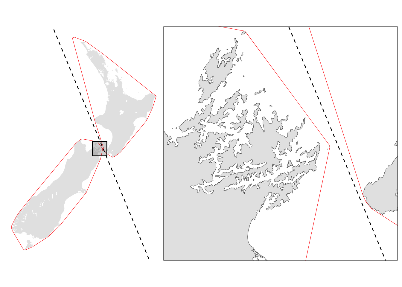
As it happens, that line is on a bearing close to north by northwest.6
So, in conclusion… East Northeast and West Southwest Islands, anyone?
Well no: Te Ika-a-Māui and Te Waipounamu will do just fine, thanks!
Were the islands ever to split (politically,7 not seismically, where the splits run in different directions) the equidistance principle would require a line be drawn more like the one I’ve worked out below using Voronoi polygons generated from points along the coastlines of the islands.
bb <- (nz |> st_bbox() + 5e4 * c(-1, -1, 1, 1)) |>
st_as_sfc()
voronoi_islands <- nz |>
st_cast("POINT") |>
st_union() |>
st_voronoi() |>
st_cast() |>
st_as_sf() |>
st_intersection(bb) |>
st_join(nz) |>
group_by(north) |>
summarise()st_voronoi extend well beyond the area of interest, so make a bounding box to clip them. The strange shenanigans with adding to the bounding box is to get properly squared off corners on extended bounding box (st_buffer’s settings don’t seem to allow for this).
And here’s a map:
g1 <- ggplot(voronoi_islands) +
  geom_sf(aes(fill = north), lwd = 0) +
  scale_fill_brewer(palette = "Set1", direction = -1) +
  geom_sf(data = nz, lwd = 0) +
  guides(fill = "none") +
  theme_void()

g2 <- ggplot(voronoi_islands) +
  geom_sf(aes(fill = north), lwd = 0) +
  scale_fill_brewer(palette = "Set1", direction = -1) +
  geom_sf(data = nz, lwd = 0) +
  guides(fill = "none") +
  coord_sf(xlim = c(1.65e6, 1.75e6), ylim = c(5.4e6, 5.5e6),
           expand = FALSE, datum = 2193) +
  theme_void()

g1 + g2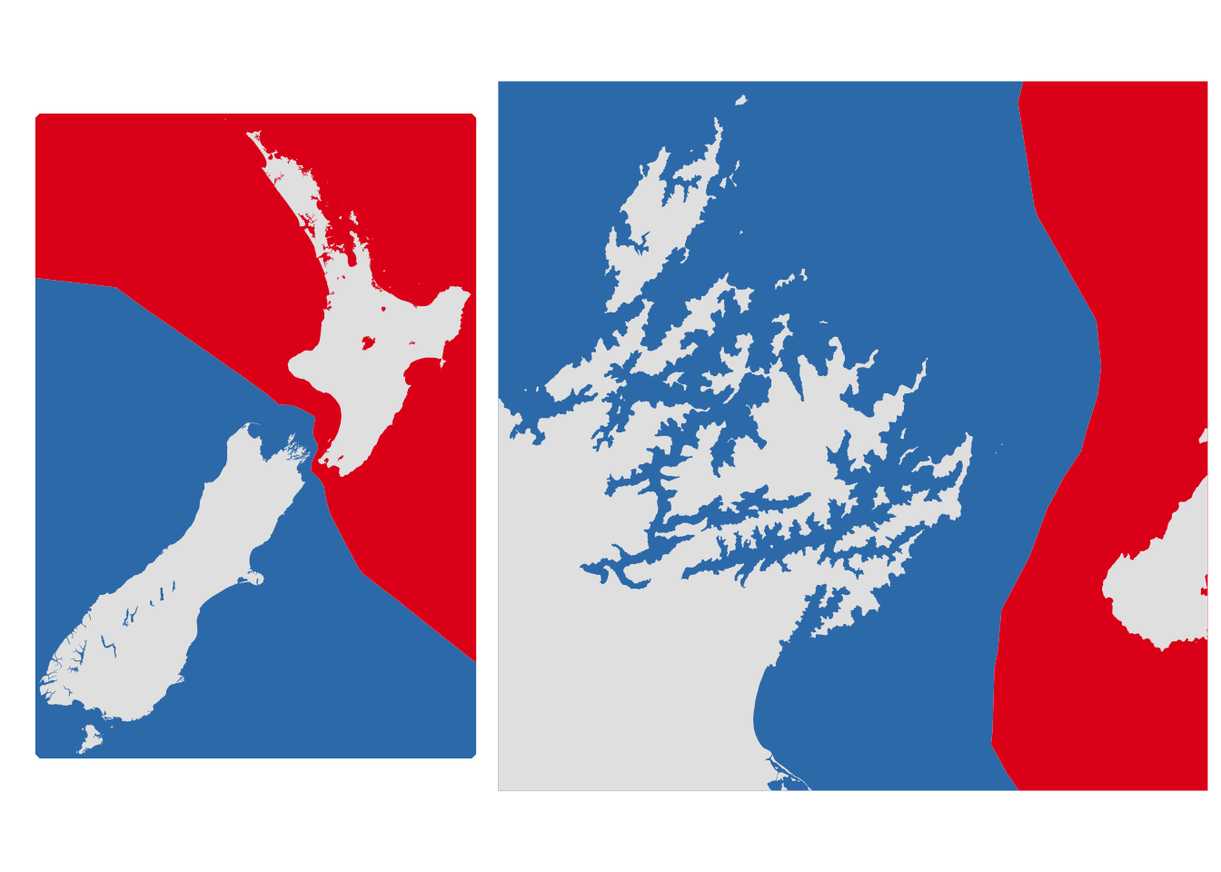
![]()
Don’t mention the Chathams. Also, I’m lumping Stewart Island / Rakiura with Te Waipounamu.↩︎
Don’t mention the football.↩︎
For what it’s worth, that observation is what I have to ‘thank’ for all this.↩︎
It may be worth noting here that a relatively common pub or Stuff quiz question concerns identifying which of a number of cities in Aotearoa New Zealand is the most easterly/westerly.↩︎
Perhaps another time… or an exercise for an enthusiastic reader.↩︎
Great movie.↩︎