How to cut a cake into four equal slices

This journey into the heart of darkness post was inspired by a LinkedIn post from Alasdair Rae linking to a map he made cutting the UK into four equal population slices. The post led to a surprising amount of complicated mathematical discussion on math reddit¹ concerning whether such a dissection should always be possible, under what conditions, and if the dissection could be extended to more slices. I think the conclusion there is that if the surface (considering the population map as a surface) is everywhere continuous—roughly speaking it varies smoothly from place to place—then such a dissection should always be possible.

This conclusion surprised me a little.² Here’s my line of thinking: I can see that there should always be a line in any given direction that halves the population. Draw a line at one side of the map area. Slide it across the map area to the other side. At the start all of the population is on one side of the line and at the end it is all on the other side of the line. If the distribution is continuous, then by the intermediate value theorem(IVT) from calculus, the line must at some point on its journey have been at a point where it cut the population exactly in half. So, pick a direction, find the line in that direction that bisects the population. The problem is that there is no guarantee that the bisector at 90° in combination with the first one will divide the population into equal quarters. It might if you ‘get lucky’, but there’s no prior reason why it would.

At this point, the mathematicians redditors invoke IVT and argue that you can choose the second line at an angle so that you do get equal quarters and then slide the crossover point and angle around until you find the place and orientation where the two lines do quadrisect³ the population.

Anyway, that’s all by way of background. Let’s see if we can find that uh… sweet spot for Aotearoa New Zealand!

library(sf)
library(dplyr)
library(tidyr)
library(stringr)
library(ggplot2)
library(scales)
library(patchwork)
library(spatstat)

1

For nicer numeric labels on some axes.

2

For nice multipanel plots.

3

For a weighted median function.

Data

I used gridded population data for New Zealand at 250m resolution. The exact dataset I used was the early release data sitting around on my hard drive from when I made this map. You can get current releases of the same data here. I converted the gridded data to an x, y, population CSV file because that’s all I need for the process I followed. I also adjusted the coordinates by centring them on their mean centre. This is to keep the coordinate values in check when we start rotating points around an origin.

pop_grid <- read.csv("nz-pop-grid-250m.csv")
cx <- mean(pop_grid$x)
cy <- mean(pop_grid$y)
pop_grid <- pop_grid |>
  mutate(x = x - cx, y = y - cy)

nz <- st_read("nz.gpkg") |>
  mutate(geom = geom - c(cx, cy))

And here is a basemap to get everyone oriented.

basemap <- ggplot(nz) + 
  geom_sf(lwd = 0) +
  geom_tile(data = pop_grid, 
            aes(x = x, y = y, fill = pop_250m_grid)) +
  scale_fill_distiller(palette = "Reds", direction = -1) +
  theme_void() +
  theme(legend.position.inside = c(0.2, 0.7),
        legend.position = "inside")
basemap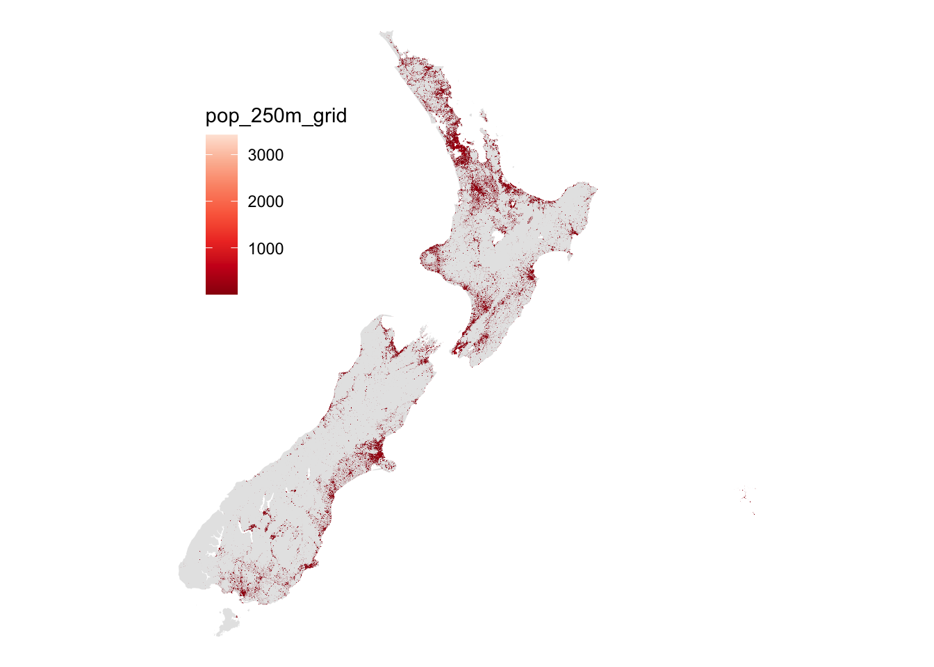

Figure 1: Base map showing distribution of Aotearoa New Zealand population.

The Chatham Islands are included here, although, since this problem is all about medians not means, it’s unlikely that outlier population makes much difference to these calculations. In any case, to a first order approximation everyone is in Auckland—that concentration of population at the narrowest point of the northern isthmus of Te Ika-a-Māui.⁴ Not really, but Auckland does loom large in what follows, as it does in cartograms of New Zealand population.

A concept of a plan of an algorithm

I briefly contemplated taking an approach similar to that outlined in the mathematical background above, but decided against it. Partly this was because building it would involve (broadly) two steps:

1. A function to find a bisector;
2. Given a bisector, a function to find another bisector at 90°, that, given the first one, quadrisects the population. This would likely involve a complicated iterative procedure sliding and rotating the pair of bisectors around until the sweet spot is found.

My short-circuiting brain kicked in after item (1) to say, “well, if you’ve found a bisector, just find all the bisectors⁵ and then test to see if any pair at 90° meet the criteria.” This would in no sense be a complete or perfect solution, but it would at least start to give some sense of how sensitive to a precise choice of locations and angles the problem is.⁶ Also, it would avoid having to deal with (2) which sounds, well… tricky.

So the plan now was

1. A function to find a bisector; and
2. Make a bunch of bisectors and test to see if any pairs at 90° are quadrisectors.⁷

This is kind of an accept-reject algorithm. It’s obviously inefficient, since we generate many incorrect candidate solutions, but if I have a reasonably quick way to find bisectors the cost of those incorrect solutions shouldn’t be too high.

Concept of a plan in place, let’s go!

A population bisector function

Here comes the science…

I could search for the bisector at a given angle, by sliding a line across a map and moving it forward or backwards depending on the population on either side of it, until I found the desired spot. That would certainly be computationally satisfying, but it’s possible to derive the line directly using a weighted median function. The weighted median of a set of numbers that have an associated weight, is the value at which the total weight associated with numbers above and below the median is equal. spatstat provides a convenient implementation, so we don’t need to do that part.

We know the slope of the desired straight line. So we rotate our x, y coordinates such that the bisector would lie flat along the horizontal axis and determine the weighted median in the vertical direction. This is the offset from the origin of the bisector perpendicular to its direction of slope. Some mathematical manipulation based on the standard form equation of a straight line \(Ax+By+C=0\) given that we know the line’s slope, and its \(x\)- and \(y\)-intercepts (based on the calculated perpendicular offset) allows us to get the \(A\), \(B\), and \(C\) coefficients we need. If the desired angle of the bisector is either horizontal or vertical no rotation is needed and we can handle these special cases easily.

So here’s code for all that, along with a couple of convenience functions to return the slope and \(y\) intercept of the straight line.

rotation_matrix <- function(a) {
  matrix(c(cos(a), -sin(a), sin(a), cos(a)), 2, 2, byrow = TRUE)
}

bisector <- function(pts, angle) {
  if (angle == 0) {
    median_y <- weighted.median(pts$y, pts$pop_250m_grid)
    A <- 0; B <- 1
    C <- -weighted.median(pts$y, pts$pop_250m_grid)
  } else if (angle == 90) {
    A <- 1; B <- 0
    C <- -weighted.median(pts$x, pts$pop_250m_grid)
  } else {
    a <- angle * pi / 180
    pts_r <- rotation_matrix(-a) %*%
             matrix(c(pts$x, pts$y), nrow = 2, byrow = TRUE)
    median_y <- weighted.median(pts_r[2, ], pts$pop_250m_grid)
    A <-  median_y / cos(a)
    B <- -median_y / sin(a)
    C <- -A * B
  }
  list(A = A, B = B, C = C)
}

get_slope <- function(straight_line) {
  -straight_line$A / straight_line$B
}

get_intercept <- function(straight_line) {
  -straight_line$C / straight_line$B
}

get_ggline <- function(straight_line, ...) {
  if (straight_line$B == 0) {
    geom_vline(aes(xintercept = -straight_line$C / straight_line$A), ...)
  } else {
    geom_abline(aes(intercept = get_intercept(straight_line), 
                    slope = get_slope(straight_line)), ...)
  }
}

1

For the horizontal bisector we want the weighted median of the y coordinates.

2

And for the vertical bisector, the weighted median of the x coordinates.

3

Rotate coordinates by the negative of the line’s slope angle so we can find the weighted median perpendicular to the line.

4

You’ll have to trust me on the calculation for A, B, and C, but keep in mind that since \(Ax+By+C=0\), the gradient of the line is given by \(-A/B\) and by inspection that’s true of these calculations, so that part checks out!

5

... means we can pass additional plot options in from the calling code.

6

When B == 0 the line is vertical so we need a geom_vline

For a given bisector we can determine which cells are either side of it by checking if \(Ax+By+C\) is positive or negative. Given that result, we can also easily determine the population either side of such a line.

get_cells_one_side_of_line <- function(pts, sl, above = TRUE) {
  if (above) {
    pts |> mutate(chosen = sl$A * x + sl$B * y + sl$C > 0) |>
      pull(chosen)
  } else {
    pts |> mutate(chosen = sl$A * x + sl$B * y + sl$C <= 0) |>
      pull(chosen)
  }
}

get_pop_one_side_of_line <- function(pts, sl, above = TRUE) {
  sum(pts$pop_250m_grid[get_cells_one_side_of_line(pts, sl, above)])
}

1

get_cells_one_side_of_line reports a logical TRUE/FALSE vector for which cells are on the requested side of the line. We do it this way to make it easier to combine the intersection of lines to determine quadrant populations later.

Sanity check

OK. So let’s see if all that has worked by running an example for a line at 30°

x30 <- bisector(pop_grid, 30)
basemap + get_ggline(x30, linetype = "dashed", lwd = 0.5) +
  guides(fill = "none")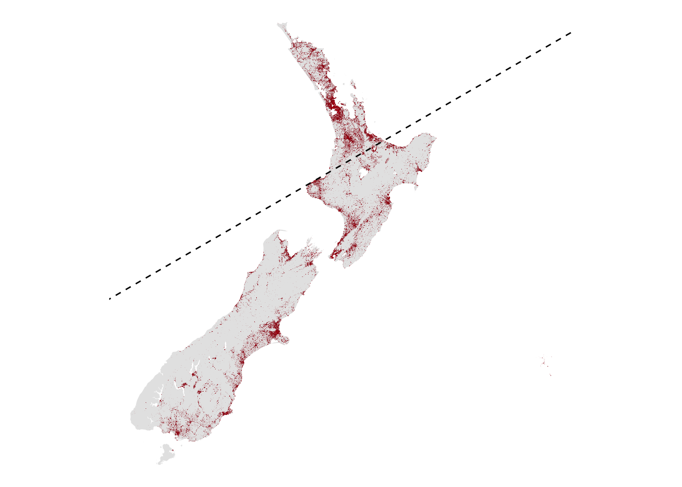

Figure 2: A map to sanity check the methods developed so far.

So we get a line at 30° as required. What are the populations either side of it?

c(get_pop_one_side_of_line(pop_grid, x30),
  get_pop_one_side_of_line(pop_grid, x30, FALSE))

[1] 2542977 2543049

Not precisely equal, but pretty close. And of course, because we are not subdividing population if the line passes through a raster cell, but assigning all of the population of a cell to whichever side of the line its centre falls in, we wouldn’t expect an exact answer.

But I wanted quadrisection

It has just occurred to me that they called this quartering in medieval times, as in “hung, drawn and quartered”… but let’s not dwell on that, and move on.

To get quadrant populations we use two lines and get the various combinations of population above/below each.

get_quadrant_pops <- function(pts, sl1, sl2) {
  above1 <- get_cells_one_side_of_line(pts, sl1)
  above2 <- get_cells_one_side_of_line(pts, sl2)
  c(sum(pts$pop_250m_grid[ above1 &  above2]),
    sum(pts$pop_250m_grid[ above1 & !above2]),
    sum(pts$pop_250m_grid[!above1 & !above2]),
    sum(pts$pop_250m_grid[!above1 &  above2]))
}

1

Get logical vectors of which cells are above the two lines.

2

And then we can combine them to get all the pairwise combinations above/below the lines and calculate the populations.

A function to plot the quadrant populations at a range of angles is convenient. Details in the cell below if you are interested.

plot_range <- function(angles) {
  bisectors      = lapply(angles     , bisector, pts = pop_grid)
  perp_bisectors = lapply(angles + 90, bisector, pts = pop_grid)
  df <- data.frame(angle = angles)
  df[, c("pop1", "pop2", "pop3", "pop4")] <-
        mapply(get_quadrant_pops, bisectors, perp_bisectors,
               MoreArgs = list(pts = pop_grid)) |> t()

  ggplot(df |> select(angle, pop1:pop4) |> 
               pivot_longer(cols = pop1:pop4)) +
    geom_line(aes(x = angle, y = value, group = name), 
              lwd = 0.2, alpha = 0.35) +
    geom_point(aes(x = angle, y = value, colour = name), 
               size = 0.5) +
    scale_colour_brewer(palette = "Set1", name = "Quadrant") +
    ylab("Estimated population") +
    scale_x_continuous(breaks = angles[seq(1, length(angles), 10)],
                       minor_breaks = angles) +
    scale_y_continuous(labels = label_number(scale_cut = cut_short_scale())) +
    theme_minimal()
}

1

Assigning the four numbers produced by get_quadrant_pops in this way seems to be the fastest approach, and preferable to a for loop. If you are writing for loops in R or Python, you are losing.

And now we can plot the quadrant populations across a range of angles from 0 to 90°.

g1 <- plot_range(-1:90) 
g1 + annotate("rect", xmin = c(-1, 76.5, 79), 
                      xmax = c(1, 78.5, 81), 
                      ymin = -Inf, ymax = Inf, 
              fill = "goldenrod", alpha = 0.3, lwd = 0)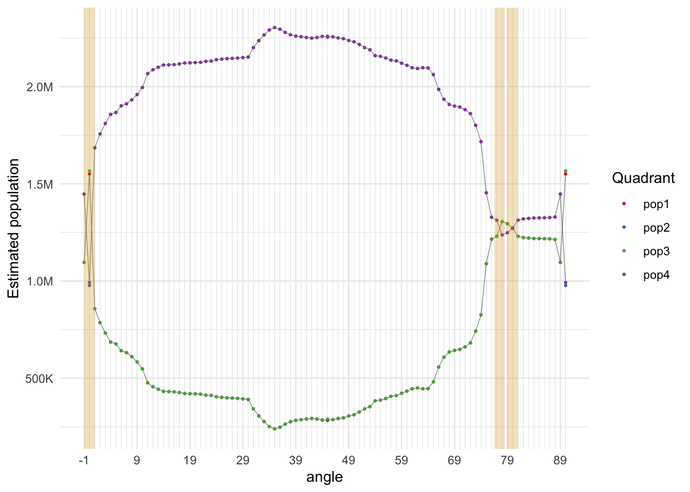

Figure 3: Variation in quadrant populations as the orientation of the first bisector is varied.

As expected these are actually two pairs of equal sums given that the two lines we are using are bisectors, so we expect diagonally opposite quadrants to have equal population, but not necessarily all four to be equal. There are three highlighted orientations where all four populations seem to converge, at around 0°, 77°, and 80°.

g2 <- plot_range(seq(-0.5,  0.5, 0.025)) + guides(colour = "none")
g3 <- plot_range(seq(  77,   78, 0.025)) + guides(colour = "none")
g4 <- plot_range(seq(79.5, 80.5, 0.025)) + guides(colour = "none")
(g2 + g3 + plot_layout(axes = "collect")) / g4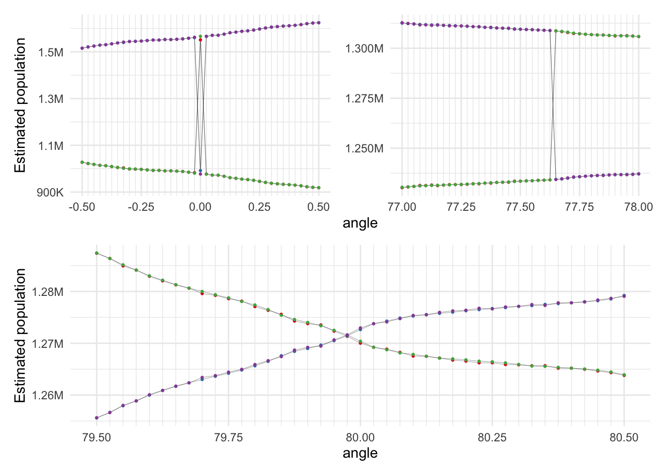

Figure 4: A closer look at the quadrant populations at angles where they appear equal.

Probably for a continuous, infinitely divisible population surface these would all be solutions to our quartering problem, but if we have a closer look (below) we can see that only the solution close to 80° actually converges for our discretised data. The other two cases have (I assume) some population grid cells jumping back and forward across our lines as we shift them slightly. On a continuous population surface I assume the behaviour at these angles would be more like the smooth variation we see in the 80° case.⁸

So finally…

The zoomed in view around 80° suggests that bisectors at angles of 79.975° and 169.975° are pretty much the ‘answer’.

Here’s a map, and the estimated populations in each quadrant, which, given the discretisation of our population data are very close to equal.

xs <- c(79.975, 169.975) |> lapply(bisector, pts = pop_grid)
x_df <- data.frame(
  slope     = xs |> sapply(get_slope), 
  intercept = xs |> sapply(get_intercept))

basemap + 
  geom_abline(data = x_df, 
              aes(slope = slope, intercept = intercept),
              linetype = "dashed", lwd = 0.5) +
  guides(fill = "none")

get_quadrant_pops(pop_grid, xs[[1]], xs[[2]])

[1] 1271354 1271442 1271630 1271600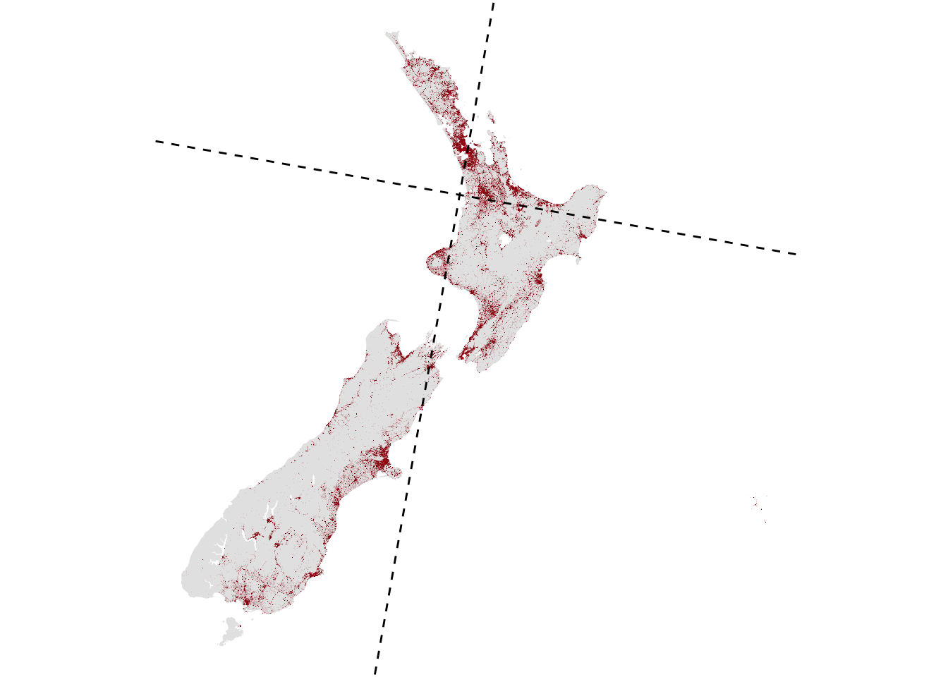

Figure 5: The best fit equal population quadrants.

It’s unsurprising as I hinted at the start, that one of the bisectors passes through Auckland, with over a third of the country’s population living there. Going anti-clockwise, starting from the northeast quadrant, these four ‘regions’ might be called Part of Auckland and Waikato-Bay of Plenty, Part of Auckland and Northland, Most of Te Waipounamu and Taranaki, and What’s Left of Te Waipounamu and Te Ika-a-Māui.

Final thoughts

Working on this problem was instructive.

Perhaps most telling is how the conclusion that a pure mathematical approach leads to—that there is always a precise solution— depends heavily on an assumption that’s difficult to realise in practice. There’s no such thing as a continuous distribution of population, so the idealised mathematics only plays out approximately in practice. Something to keep in mind in many problem settings. Even so, the mathematics is useful: it tells us that there should be a solution even if that seems unlikely given real world data.

To find that ‘precise’ solution, we’d have to do the dissections in a way that yielded continuously varying estimates of the populations either side of a line as it is infinitesimally shifted around. For example, we could use an areal interpolation method, assigning the proportion of population in a grid cell based on the fraction of its area on each side of the line. This seems likely to be quite a lot slower than my admittedly approximate approach.

A further thought is that lurking in here are almost certainly the ingredients for a treemap/quadtree approach to cartograms. This is not an entirely new idea. For example in this paper

Slingsby A, J Wood, and J Dykes. 2010. Treemap Cartography for showing Spatial and Temporal Traffic Patterns. Journal of Maps 6(1) 135-146. doi: 10.4113/jom.2010.1071

spatialised treemaps are applied to visualize complex data.

I am envisaging bisecting horizontally, then bisecting each half vertically, then each quarter horizontally, and so on. The resulting rectangular regions would be of equal population, and could be rescaled to be of equal size after each cut. Something like that. The idea definitely needs work, but I think it has potential.

But that’s another puzzle for another time.

Footnotes

1. Yes, that’s a thing.

2. Notwithstanding the counterintuitive wonders of the ham sandwich theorem invoked by many of the math redditors.

3. Yes, it’s a word, I checked.

4. Back in the day, this made a lot of sense as an overland shortcut between a harbour on the Pacific and another on the Tasman. Now as a place to concentrate your population it’s not so obviously a good choice.

5. At some angular resolution.

6. I’d call it an agile approach if I were being kind. A little more seriously, I’d call it getting a feel for the problem before bothering to tackle it in full.

7. I’m less certain this is a word.

8. Probably… I can’t be absolutely certain of this. We’d have to look more closely to investigate which grid cells are ‘jumping around’ at these values to confirm this assumption.