Code
import requests
import io
import pandas as pd
import geopandas as gpd
import city2graph as c2g
import osmnx as ox
import foliumIn this post, I revisit my very earliest academic contribution,1 which demonstrated how to generate isochrone maps in a GIS based on public transport timetable data. An isochrone is a line delineating a set of points reachable in some set time from some starting location, given the transport options available. This is a notion that has by now become a lot more familiar than it was back then, perhaps most especially via the (ahem) magnificent mapnificent.net website.
In my masters thesis on which that paper was based, I did a lot of this by hand. I started by grabbing a huge number of paper bus timetables from the central station in Glasgow.2 In the absence of reliable data on where bus stops were, and with insufficient time to travel every bus route and geocode them, I used the timetables to generate ‘fake’ bus stops by running shortest path analysis between the end points of each route via some known intervening locations, determined from the timetables and a handy-dandy copy of the AZ Street Atlas of Glasgow Hamilton Motherwell Paisley.3 A further simplification was to focus on off-peak times only, and to use only bus route frequencies not timetabled arrival and departure times.
Anyway, I used all this to generate some truly horrible maps. The colour scheme I used boggles my mind. Let’s just say I am retrospectively grateful that the reference electronic versions of the maps in the literature are in greyscale.4
All of which brings me back to this post, where using the recently released city2graph5 module and the by now venerable osmnx6 I make some street based, combined bus and walking isochrones for my local Wellington bus route, the number 7.
First up, we need a bunch of python modules. requests and io are needed to pull the Wellington GTFS feed from its online home; pandas and geopandas for processing the tabular data; city2graph and osmnx for the core processing; and folium for web map outputs.
import requests
import io
import pandas as pd
import geopandas as gpd
import city2graph as c2g
import osmnx as ox
import foliumYou can do many things with city2graph. Here, the main task is to process General Transit Feed Specification (GTFS) data into a format suitable for our analysis. First, here’s a URL for the Wellington GTFS feed.
gtfs_url = "https://static.opendata.metlink.org.nz/v1/gtfs/full.zip"As I noted in my masters thesis public transport systems are complicated. Very complicated. At the time the Glasgow region’s system apparently had as many as 12,000 transit routes, at least when viewed from the perspective of the people running the system, who consider every minor variation of a route to be different, where variation might include running on different days, at different times, or following a slightly different route. As a transport user we tend to think in terms of the number 7 bus, but for the transport system operator it’s not as simple as that: the number 7 might refer to several hundred possible trips, in several subtly different varieties.
GTFS reflects this complexity with the full specification requiring minimally 7 files setting out agencies, routes, trips, stops, stop-times, a calendar, and calendar dates, and with an additional optional 15 files that provide further details of fares, fare transfer rules, and a great deal more besides.
city2graphcity2graph happily parses all this complexity into a dictionary of tables which provide us with all the information we need for the present analysis at least. It’s so easy, that the trickiest part of the line of code below was working out how to get it to read from an online source.
gtfs = c2g.load_gtfs(io.BytesIO(requests.get(gtfs_url).content))I’ll focus on the high frequency route 7 that passes through Brooklyn, the suburb where I live, into central Wellington (direction 1).
route = "7"
direction = "1"
I use this information to get a route_id.
route_id = (
gtfs["routes"]
.query("route_short_name == @route")
.route_id
.iloc[0]
)
route_idpandas table query.
'70'And then use this to retrieve trip IDs that relate to this route.
trip_ids = (
  gtfs["trips"]
  .query("route_id == @route_id & direction_id == @direction")
  .sort_values(["service_id", "trip_id"])
  .loc[:, ["trip_id"]]
)
trip_ids.shape[0], trip_ids.head()
(152,
trip_id
7019 7__1__700__TZM__102__2__102__2_20250817
5703 7__1__100__TZM__102__7__102__7_20250817
4691 7__1__116__TZM__102__7__102__7_20250817
47 7__1__400__TZM__103__3__103__3_20250817
7397 7__1__450__TZM__103__3__103__3_20250817)There are actually 152 of these! For lack of anything better, I’m just going to focus on the first, and retrieve the associated stop times. These are the timetabled arrival times at each stop along the route for a particular trip.
trip_id = trip_ids.trip_id.iloc[0]
stop_times = (
  gtfs["stop_times"]
  .query("trip_id == @trip_id")
  .loc[:, ["trip_id", "stop_id", "arrival_time"]]
  .sort_values("trip_id")
)
stop_times.head(),
( trip_id stop_id arrival_time
255719 7__1__700__TZM__102__2__102__2_20250817 7730 07:35:00
255741 7__1__700__TZM__102__2__102__2_20250817 5012 07:54:24
255740 7__1__700__TZM__102__2__102__2_20250817 5010 07:53:51
255739 7__1__700__TZM__102__2__102__2_20250817 5008 07:52:27
255738 7__1__700__TZM__102__2__102__2_20250817 7708 07:50:55,)This table gives us a stop_id and associated arrival time on this particular trip on the number 7, and we can use that information to build an associated set of isochrones.
Below, I use pandas’ facility with date and time formats, to convert the arrival times into a series of ‘time remaining’ values. For some allowed period of time, which I here choose to be 30 minutes, I set the end time of the isochrone to be 08:05 (since the bus sets off at 07:35). The arrival time at each stop on the route admits some further travel time before 08:05, which is calculated as a ‘time remaining’.
end_time = pd.to_datetime("08:05:00", format = "%X")
times_remaining = (
stop_times
.assign(
time_remaining = (
end_time - pd.to_datetime(stop_times.arrival_time, format = "%X"))
.dt.seconds)
.loc[:, ["stop_id", "time_remaining"]]
)
times_remaining.head(),( stop_id time_remaining
255719 7730 1800
255741 5012 636
255740 5010 669
255739 5008 753
255738 7708 845,)This code is where, if we wanted to make a set of isochrones with different total available times, we could do so by iterating over a series of end_time values, calculating the time remaining, and if applicable dropping stops where there was no time or only negative time remaining (i.e. it takes longer to get to them than the time budget allows).
Given the time remaining at each stop, we can use a simple buffering method to produce a circular area centred on each stop which is the potentially reachable area around that stop, assuming a walking speed of 1m/s and an ability to pass through walls, trees, and anything else in between (i.e., this ignores things like footpaths, roads, and so on).
route_stops = (
  gtfs["stops"]
  .merge(times_remaining)
  .sort_values("time_remaining", ascending = False)
)
bubbles = [s.buffer(d)
           for s, d in zip(route_stops.geometry.to_crs(2193),
                           route_stops.time_remaining)]

isochrone_bubbles = gpd.GeoDataFrame(
  geometry = gpd.GeoSeries(bubbles), crs = 2193)

isochrone_bubbles.plot(alpha = 0.1).set_axis_off()
We can think of the ‘bubble’ isochrones as a best-case scenario. But in the real world we have to pound the pavement and walk along approved paths and this will generally mean that progress is slower than the straight line distances of simple buffers imply. This is where osmnx comes in.
First, it’s useful to make a bounding box from the bubble isochrone, since it defines the farthest possible progress at every location, and use this to extract a street graph using osmnx’s graph.graph_from_bbox() method.
bb = [float(x)
      for x in isochrone_bubbles.to_crs(4326).total_bounds]
G = ox.graph.graph_from_bbox(bb, network_type = "walk",
                             simplify = False)
Now, based on this graph, we can determine for each stop, the nearest node on the street network.
nearest_nodes = ox.distance.nearest_nodes(G,
  [p.x for p in route_stops.geometry],
  [p.y for p in route_stops.geometry])
And based on these nodes, we can pull subgraphs of the street graph that are within a distance along the street network limited by the time remaining at each stop, again assuming progress at 1m/s.7
isochrone_streets = (
  gpd.GeoDataFrame(
    geometry = gpd.GeoSeries(pd.concat([
      ox.convert.graph_to_gdfs(
        ox.truncate.truncate_graph_dist(G, node, dist),
        nodes = False).geometry
      for node, dist in zip(
        nearest_nodes,
        route_stops.time_remaining)]).union_all(),
    crs = 4326)
  ).to_crs(2193)
)
isochrone_streets.plot().set_axis_off()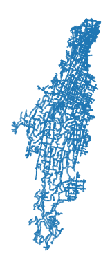
We can also derive an approximate polygon outlining the street network using the relatively recent concave_hull addition to geopandas.
isochrone_approx = (
  isochrone_streets
  .concave_hull(ratio = 0.025)
)Now we’re ready to assemble all these layers into a composite map of the number 7 bus route.
m = folium.Map(
  tiles = None,
  zoom_start = 13, max_bounds = True,
  location = [(bb[0] + bb[2]) / 2, (bb[1] + bb[3]) / 2],
  min_lon = bb[0], min_lat = bb[1],
  max_lon = bb[2], max_lat = bb[3]
)

folium.TileLayer("CartoDB Positron", overlay = True).add_to(m)

isochrone_bubbles.explore(
  m = m, name = "Walk time circles", tooltip = False,
  style_kwds = dict(fill = False, color = "black", weight = 0.35))

isochrone_approx.explore(
  m = m, name = "Approximate isochrone", tooltip = False,
  style_kwds = dict(color = "red", fill = False, weight = 3))

isochrone_streets.explore(
  m = m, name = "Streets isochrone", tooltip = False,
  style_kwds = dict(color = "orange", weight = 1))

route_stops.explore(
  m = m, name = "Stops", tooltip = "stop_name",
  style_kwds = dict(color = "red", fill = False, radius = 6))

folium.LayerControl().add_to(m)
mThis map shows, in a number of different ways the places reachable by way of the number 7 bus and walking, within 30 minutes starting from the moment at which you choose to board the 07:35 starting at the Kingston end of the route or not.8
At the Kingston end, if you were able to fly, you could get a long way in 30 minutes (as shown by the large circles). In practice, on the ground, the options are more limited because, in common with many places in Wellington, the roads just come to an end.
If you alight from the bus halfway into town you have time to walk a reasonable distance from your stop and this is reflected in the ‘widening’ out of the street based isochrone.
If you don’t get off the bus until near the terminus at Wellington Station, then your options on foot narrow down to only a small area close to the station.
In my thesis I attempted to model transfers between buses, and doing that here would get complicated pretty quickly, but not outrageously so. And of course, in my thesis I only modelled the off-peak timetable, and approximately at that. With the detailed data available from GTFS I could have been a lot more ambitious.9
city2graph GTFS goodnessHere’s an example of something you can do with GTFS using city2graph that would be excruciatingly painful to do manually working with individual GTFS files. The travel_summary_graph() method takes a stack of GTFS files and subjects them to further analysis, determining the average time taken across all trips to get between consecutive stops on the network.
pts, segments = c2g.travel_summary_graph(gtfs)
pts = pts.reset_index()
segments_m = segments.to_crs(2193)
segments_m.head(),
( mean_travel_time frequency \
from_stop_id to_stop_id
0001 1800 257.000000 20
0002 1806 70.800000 20
1905 56.000000 20
0003 1817 27.400000 20
1916 127.238095 21
geometry
from_stop_id to_stop_id
0001 1800 LINESTRING (1804586.846 5436469.543, 1806080 5...
0002 1806 LINESTRING (1798074.727 5442644.393, 1797469.9...
1905 LINESTRING (1798074.727 5442644.393, 1798720.0...
0003 1817 LINESTRING (1799389.472 5445379.483, 1799729.9...
1916 LINESTRING (1799389.472 5445379.483, 1797980.0... ,)This allows me to explore one of my local niggles with the number 7 bus, which is the seemingly stupidly high density of stops in Brooklyn. These involve the bus stopping at less than 60 second intervals three times in the so-called ‘village’, which is really barely more than a hundred metres or so of shops and take aways. I suspect this annoys drivers at least as much as it annoys me.10
Querying the analysis results for stops less than 200 metres apart which are also less than 60 seconds apart allows us to map the offenders. Suffice to say, Brooklyn and the No. 7 are not alone in this.
segments_m = (
  segments_m
  .assign(length  = segments_m.geometry.length.round(0),
          mean_travel_time = segments_m.mean_travel_time.round(0))
  .query("length < 200 & mean_travel_time < 60")
)
(segments_m
  .explore(tiles = "CartoDB Positron",
           style_kwds = dict(color = "red", weight = 3))
)![]()
O’Sullivan D, A Morrison and J Shearer. 2000. Using desktop GIS for the investigation of accessibility by public transport: an isochrone approach. International Journal of Geographical Information Science 14(1) 85-104.↩︎
This was a time when such things still existed. I guess they must have assumed I was a public transport timetable nut enthusiast.↩︎
Surprisingly, you can still get one of these.↩︎
If you’re interested in the horrors I reserved colour printing for in the thesis itself, then take a look here.↩︎
Sato Y. 2025. city2graph: Transform geospatial relations into graphs for spatial network analysis and Graph Neural Networks doi:10.5281/zenodo.15858845.↩︎
Boeing G. 2025. Modeling and Analyzing Urban Networks and Amenities with OSMnx. Geographical Analysis.↩︎
If you are familiar with Wellington’s rugged terrain, you’ll know this is a generous assumption. In principle, it wouldn’t be difficult to include street slope, but that’s another question, for another day.↩︎
That’s where the metaphorical sliding doors come in, even if buses don’t generally have actual sliding doors.↩︎
Saying that, GTFS timetable data is theoretical, not actual, and the difference may matter greatly, a topic explored in this paper: Wessel N and S Farber. 2019. On the accuracy of schedule-based GTFS for measuring accessibility. Journal of Transport and Land Use. 12(1) 475-500.↩︎
Saying which, it’s a collective action problem. Riders could choose collectively, somehow, not to use one or more of the pretty much redundant stops, but we don’t. And I include myself in that number. And we are probably all equally annoyed about it.↩︎