Raster really is faster – Geospatial Stuff

I’ve been asked relatively often when or if there will be a third edition of Geographic Information Analysis. Notwithstanding how happy it makes me (and Dave Unwin) to know that people find that book valuable, it’s sadly unlikely. Dave has retired, my relationship to academia is not what it was, and there’s also the aggravation associated with Wiley holding the copyright. Dave and I think that their approach to books like this is out of date, not to mention somewhat predatory price-wise, and we’d like to be able to offer a cheaper (perhaps even free) product,¹ but Wiley won’t surrender the copyright and we’re stuck.

As a limited alternative, I thought I’d write some posts providing code implementing ideas from the book. Robert Hijmans has already done this to a large extent but there’s no harm in repetition, and I expect I’ll wind up presenting different perspectives (or at the very least datasets).

In Chapter 1 Geographic Information Analysis and Spatial Data, in a section called Objects Might Have Fractal Dimension² we presented fractal dimension as one instance of the scale dependence of spatial data. Herewith, some R code exploring that idea³ and incidentally, as the title implies, showing some of the differences between vector and raster data.

Measuring fractal dimension

We need some packages - the usual suspects, really.

Code

library(sf)
library(units)
library(ggplot2)
library(dplyr)
library(stringr)

Since fractal dimension is determined from a log-log relationship it is convenient to be able to generate sequences like 1, 2, 5, 10, 20, 50,… and so on, so here are a couple of functions for doing just that.

Code

round_to_1_2_5 <- function(x, offset = 0) {
  offset <- ifelse(offset > 0, 1, ifelse(offset < 0, -1, 0))
  decade <- c(1, 2, 5) * 10 ^ floor(log10(x))
  idx <- sum(x >= decade)
  if (idx == 3 & offset >=  1) return(decade[1] * 10)
  if (idx == 1 & offset <= -1) return(decade[3] / 10)
  decade[idx + offset]
}

get_decades <- function(low = 1, high = 1000, 
                        offsets = c(0, 0)) {
  lo <- round_to_1_2_5(low, offsets[1])
  hi <- round_to_1_2_5(high, offsets[2])
  steps <- c(1, 2, 5)
  decades <- c()
  for (decade in floor(log10(lo)):ceiling(log10(hi))) {
    decades <- c(decades, steps * 10 ^ decade)
  }
  decades[which(decades >= lo & decades <= hi)]
}

The measurement process

Next up, the main event, at least in vector-land.

Fractal dimension reflects how the apparent length of a line (or area of a region) seems to increase the more closely we look. In practical terms in the case of measuring the length of (as here) coastlines, this manifests as follows. Take a measuring stick of some ‘resolution’ (i.e. length), say 1km, repeatedly fit it to the coastline, and count how many times it fits. A long measuring stick will miss lots of nooks and crannies. A shorter one will fit into many more, and so, as the size of your measuring stick shrinks, the measured length of the coastline will grow.

It turns out that the relationship between measuring stick length, \(m\), and the number of times it will fit the line you are measuring, \(N\) scales according to \(\log{N}\propto\log{m}\), and the ratio of the logarithms of those two values, is the fractal dimension, \(D\), that is

\[ \log{N}=-D\log{m}+c \] In other words, the negative slope of a log-log plot showing the relationship between \(N\) and \(m\) gives us the fractal dimension. The more ‘crinkly’ a line the more rapidly \(N\) will increase as \(m\) shrinks. In the extreme case of a space-filling curve,⁴ \(D=2\) and the line is in effect an area!

Anyway, to return to the issue at hand, the function below identifies the ‘measuring points’ at which a yardstick of some specified length will touch a supplied line. Hover over the circled numbers at the side for details.

Code

get_measuring_pts <- function(shape, yardstick = 1e3) {
  next_point <- shape |> 
    st_cast("POINT") |> 
    slice(1)
  measuring_pts <- list(next_point)
  next_position <- 0
  last_position <- -1
  while (next_position > last_position) {
    last_position <- next_position
    buffer_line <- next_point |>
      st_buffer(yardstick) |> 
      st_boundary()
    next_points = buffer_line |>
      st_intersection(shape) |>
      st_cast("POINT")
    next_positions = st_line_project(
      shape |> st_as_sfc(),
      next_points |> st_as_sfc(),
      normalized = TRUE)
    if (any(next_positions > last_position)) {
      next_position = min(next_positions[
        which(next_positions > last_position)])
      next_point <- next_points |>
        slice(which(next_positions == next_position))
      measuring_pts[[length(measuring_pts) + 1]] <- next_point
    } else { break }
  }
  measuring_pts |> 
    lapply(data.frame) |> 
    bind_rows() |> 
    st_as_sf(crs = st_crs(shape))
}

1: shape is an sf dataset containing a single LINESTRING geometry, and yardstick is the length of the measuring stick—its resolution.
2: We start from the first point in the line.
3: Initialise a list to record the points at which the yardstick touches the line with the first point.
4: next_position and last_position are how far along the line measurement has progressed. For a closed line, when next_position is less than last_position we’ve looped back around to the start and are done.
5: Use a linear buffer, not a polygon, so that the intersections with the line are a set of points.
6: Get all the potential next points: these are where the line buffer intersects the shape.
7: Get how far along the shape the next points are.
8: If none of the next positions are further along the shape than the last position, then we are done.
9: Pick the closest intersection point as the next point and add it to the list of measuring points.
10: Convert the list of points to an sf dataset, and return.

We also need a function to convert the points to a polygon.

Code

get_approx_polygon <- function(mpts) { 
  mpts |> 
    st_combine() |>
    st_cast("LINESTRING") |>
    st_cast("POLYGON") |>
    as.data.frame() |> 
    st_as_sf()
}

A test of the measurement method

Now, if we load up some data we can see what this looks like.

Code

nz <- st_read("nz-large.gpkg") 

nz_no_holes <- nz |> 
  st_cast("POLYGON") |> 
  mutate(geom = st_exterior_ring(geom))

nz_largest_islands <- nz_no_holes |>
  mutate(area = st_area(geom) |> drop_units()) |>
  arrange(desc(area)) |>
  select()

waiheke <- nz_largest_islands |> 
  slice(8) |>
  st_cast("LINESTRING")

The eighth largest of the Aotearoan islands is Waiheke, and for it, a resolution of 1km provides a reasonable test of the yardstick measurement procedure.

Code

yardstick <- 1000
measuring_pts <- get_measuring_pts(waiheke, yardstick)
approximate_island <- get_approx_polygon(measuring_pts)

ggplot() +
  geom_sf(data = waiheke |> st_cast("POLYGON"), 
          fill = "#cccccc", colour = NA) +
  geom_sf(data = approximate_island,
          fill = "NA", colour = "blue", lwd = 0.65) +
  geom_sf(data = measuring_pts,
          colour = "red") +
  geom_sf(data = measuring_pts |> st_buffer(yardstick),
          fill = NA, colour = "red") +
  theme_void()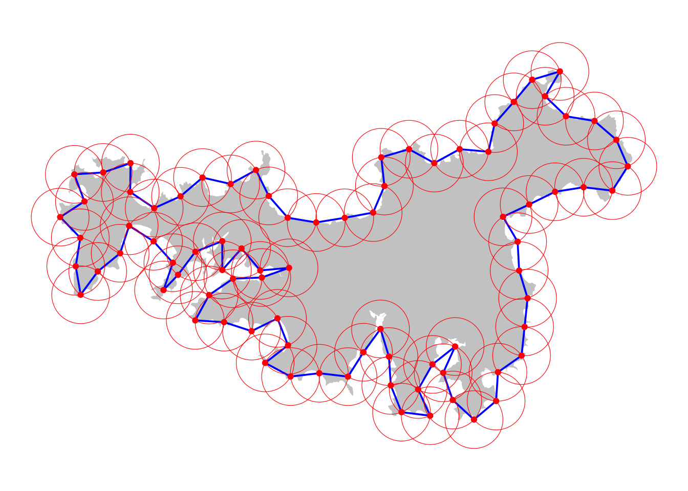

Figure 1: Illustrating the method applied to Waiheke

Hopefully, the figure shows how measuring the coastline at a single resolution works. Starting at some point (one of the red dots). We repeatedly find the closet point further around the coastline that is 1km distant. Counting up how many times we can do this gives an estimate at the current resolution of the length of the coastline, and also gives us the number \(N\) of yardsticks at this resolution.

Estimating fractal dimension

Method 1: using several measuring sticks

Having established that the method works, we can use it to assemble a series of measurements and estimate the fractal dimension. For this, we’ll use the North Island, Te Ika-a-Māui. We also set up a series of yardsticks to apply.

Code

te_ika_a_maui <- nz_largest_islands |> 
  slice(2) |>
  st_cast("LINESTRING")
yardsticks <- get_decades(5000, 200000)

Now, we loop over the resolutions, and assemble the resulting approximating polygon, along with the number of contact points in the measurement process.

Code

df <- yardsticks |> 
  lapply(get_measuring_pts, shape = te_ika_a_maui) |>
  lapply(get_approx_polygon) |>
  bind_rows() |>
  mutate(yardstick = yardsticks,
         yardstick_name = ordered(
          str_c(yardstick / 1000, " km"),
          levels = str_c(yardstick / 1000, " km")),
         coastline = geometry |>
           st_boundary() |> 
           st_length() |> 
           drop_units(),
         n = coastline / yardstick)

1: Make a list by applying the get_measuring_pts function to the set of yardstick lengths.
2: Convert to approximate polygons (for mapping later).
3: Since the measuring stick doesn’t fit an exact number of times, we may as well measure the exact coastline length…
4: … and the exact (non-integer) number of measuring sticks.

The linear fit between the log of the number of yardsticks and the log of the yardstick length is easily modelled, and the negative coefficient is our estimate of the fractal dimension, which in this case comes to 1.203. A fractal dimension of around 1.2 is about what we would expect for an extensive coastline like this, with some very crenellated sections and other relatively smooth stretches.

Code

lm(log10(n) ~ log10(yardstick), data = df)


Call:
lm(formula = log10(n) ~ log10(yardstick), data = df)

Coefficients:
     (Intercept)  log10(yardstick)  
           7.336            -1.203

A log-log plot makes the relationship clear.

Code

y_breaks <- get_decades(min(df$n), max(df$n), c(-1, 1))
ggplot(df, aes(x = log10(yardstick), y = log10(n))) +
  geom_point() +
  geom_smooth(formula = y ~ x, method = "lm") +
  scale_x_continuous(breaks = log10(yardsticks),
                     labels = yardsticks) +
  xlab("Yardstick length, km") +
  scale_y_continuous(breaks = log10(y_breaks),
                     labels = y_breaks) +
  ylab("Number of yardsticks") +
  theme_minimal()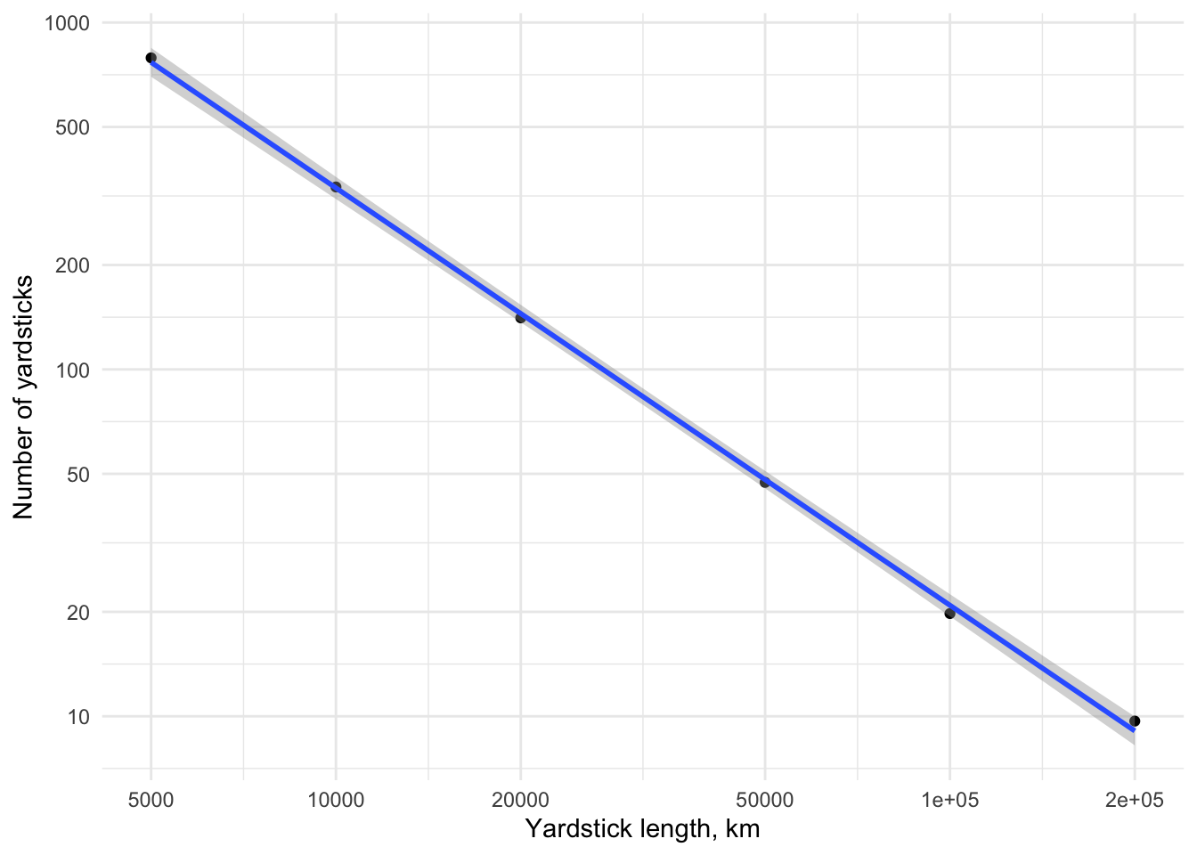

Figure 2: The relationship between measuring stick length and the number of measuring sticks for Te Ika-a-Māui.

We can see how the measurement process changes, and why the long yardsticks underestimate badly in the sequence of maps below.

Code

ggplot() +
  geom_sf(data = te_ika_a_maui |> st_cast("POLYGON"), colour = NA) +
  geom_sf(data = df, lwd = 0.5) +
  facet_wrap( ~ yardstick_name, ncol = 3) +
  theme_void()

Figure 3: Map sequence for the six coastline measurements on which the estimated fractal dimension is based.

Method 2: raster is faster

The above is all very well, but OMG it is sloooooowwwwwwww… A much quicker approach is possible using a raster method.

We replace the measuring stick with raster cells, and simply count how the number of cells that the coastline passes through changes with the resolution of the cells. While the code below converts the raster representation to an xy-table, this is only done to make it easier to produce the small multiple map in ggplot.

Code

library(terra)

sv <- te_ika_a_maui |> as("SpatVector")
yardsticks2 <- get_decades(200, 200000)
sums <- c()
rasts <- list()
for (res in yardsticks2) {
  r <- sv |>
    rasterize(rast(sv, res = res)) |>
    terra::as.data.frame(xy = TRUE) |>
    mutate(resolution = res,
           resolution_label = ordered(
             str_c(resolution / 1000, " km"),
             levels = str_c(yardsticks2 / 1000, " km")))
  rasts[[length(rasts) + 1 ]] <- r
  sums <- c(sums, r |> pull(3) |> sum())
}
df2 <- data.frame(yardstick = yardsticks2, n = sums)
lm(log(n) ~ log(yardstick), data = df2)


Call:
lm(formula = log(n) ~ log(yardstick), data = df2)

Coefficients:
   (Intercept)  log(yardstick)  
        17.274          -1.224

Note that because this method is much faster,⁵ we can extend the range of resolutions used to a lower value of only 200m without difficulty (lower still would be fine too, although you would then struggle to see the resulting rasterized maps of the coastline at all).

Code

y_breaks <- get_decades(min(df2$n), max(df2$n), c(-1, 1)) 
ggplot(df2, aes(x = log10(yardstick), y = log10(n))) +
  geom_point() +
  geom_smooth(formula = y ~ x, method = "lm") +
  scale_x_continuous(breaks = log10(yardsticks2),
                     labels = yardsticks2 / 1000) +
  xlab("Yardstick length, km") +
  scale_y_continuous(breaks = log10(y_breaks),
                     labels = y_breaks) +
  ylab("Number of yardsticks") +
  theme_minimal()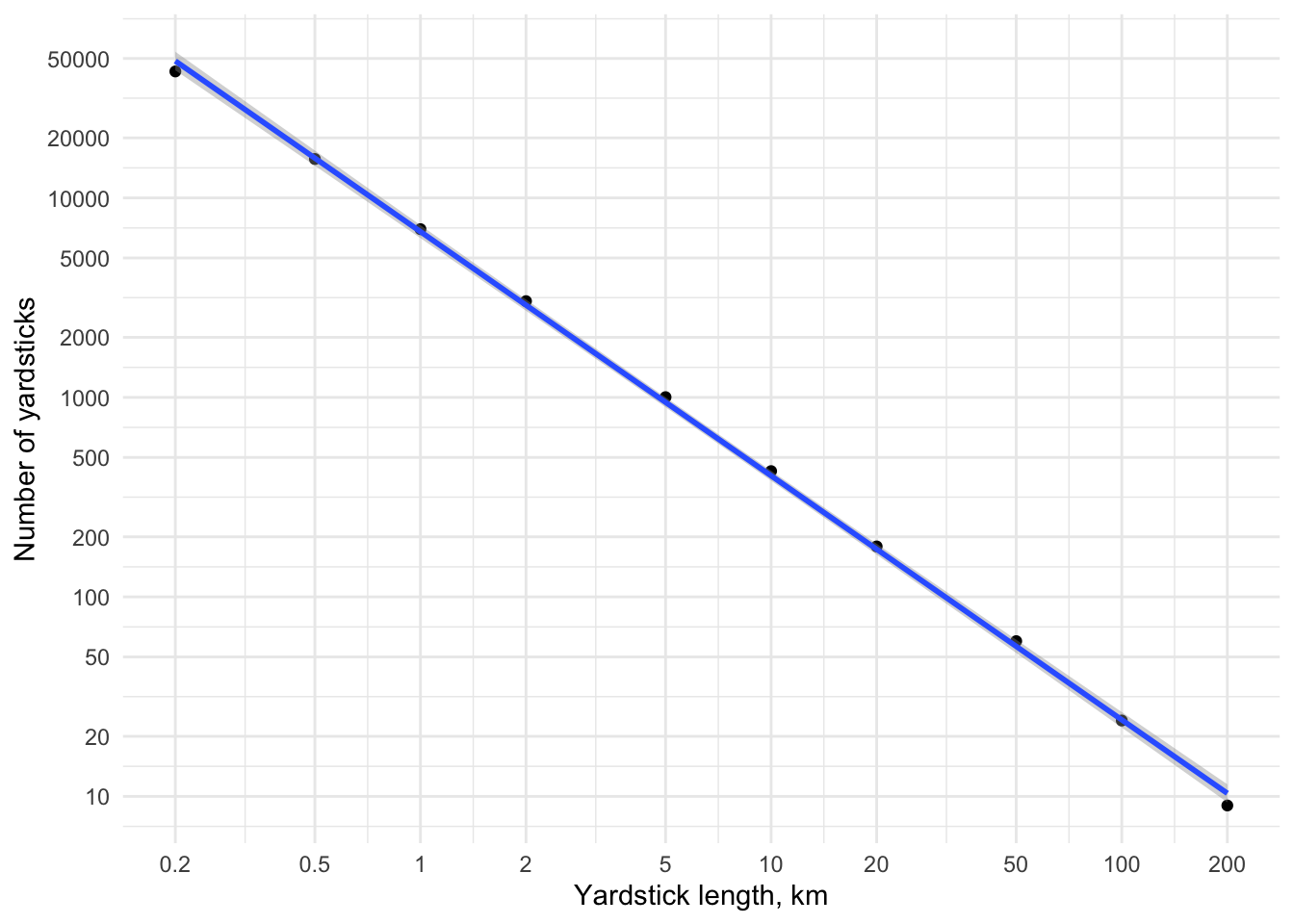

Figure 4: Log-log plot of results from the raster-based method.

The resulting estimate is similar to that produced by the vector method. It’s not at all obvious which is ‘more correcter’.⁶ We can also get a map sequence of the progressive degradation of the coastline measurement as the raster resolution coarsens.

Code

xy_df <- bind_rows(rasts)
ggplot(xy_df) +
  geom_tile(aes(x = x, y = y,
                width = resolution, height = resolution)) +
  coord_sf() +
  facet_wrap( ~ resolution_label, ncol = 5) +
  theme_void()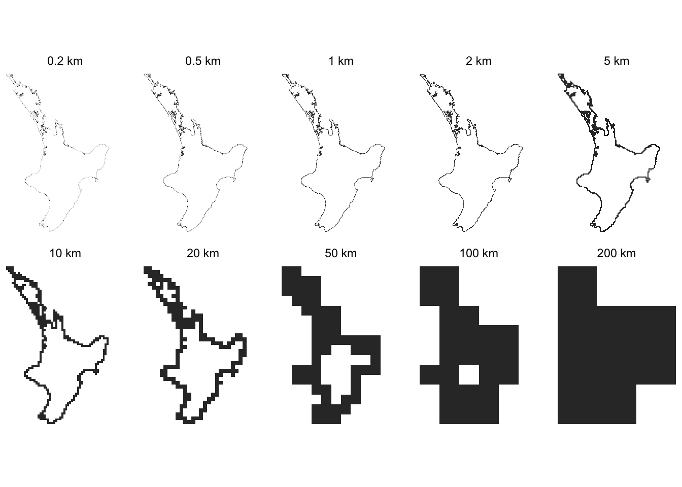

Figure 5: Map sequence for the raster-based estimation method

Method 3: using a vector (hex) grid

This section is by way of an addendum really. The success of the raster method got me wondering if an alternative vector grid method might be quicker than the original approach. The answer is… it works, and it is quicker than the first vector method above, but it’s still a lot slower than the raster method.

It’s nice that it’s easy to make the grid hexagon-based, which might assuage the concerns of those worried about the different distances diagonal and face-to-face across square grid cells.

Code

yardsticks3 <- get_decades(5000, 200000)
counts <- c()
hex_sets <- list()
for (yardstick in yardsticks3) {
  hex_centres <- te_ika_a_maui |>
    st_make_grid(cellsize = yardstick,
                 square = FALSE,
                 what = "centers") |>
    st_as_sf() |>
    st_filter(te_ika_a_maui,
              .predicate = st_is_within_distance,
              dist = yardstick / 2) |>
    mutate(cellsize = yardstick,
           cellsize_label = ordered(
             str_c(cellsize / 1000, " km"),
             levels = str_c(yardsticks3 / 1000, " km")))
  hex_sets[[length(hex_sets) + 1]] <- hex_centres
  counts <- c(counts, dim(hex_centres)[1])
}
df3 <- data.frame(yardstick = yardsticks3, n = counts)
lm(log(n) ~ log(yardstick), data = df3)

1: square = FALSE means the grid is hex-based, and what = "centers" that we get cell centres not the polygons.
2: Note that the spatial filter is based on half the distance between the centres, cells with centres within that distance of the coastline will intersect it.


Call:
lm(formula = log(n) ~ log(yardstick), data = df3)

Coefficients:
   (Intercept)  log(yardstick)  
        16.983          -1.187

Again, a similar estimate. And here are the corresponding log-log plot and map sequences.

Code

y_breaks <- get_decades(min(df3$n), max(df3$n), c(-1, 1))
ggplot(df3, aes(x = log10(yardstick), y = log10(n))) +
  geom_point() +
  geom_smooth(formula = y ~ x, method = "lm") +
  scale_x_continuous(breaks = log10(yardsticks3),
                     labels = yardsticks3 / 1000) +
  xlab("Yardstick length, km") +
  scale_y_continuous(breaks = log10(y_breaks),
                     labels = y_breaks) +
  ylab("Number of yardsticks") +
  theme_minimal()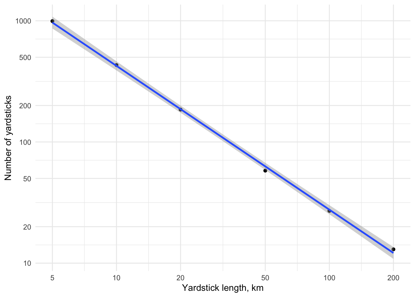

Figure 6: Log-log plot of the hex grid centres based method.

Code

centres_df <- bind_rows(hex_sets)
ggplot() +
  geom_sf(data = te_ika_a_maui |> st_cast("POLYGON"), colour = NA) +
  geom_sf(data = centres_df, size = 0.2) +
  facet_wrap( ~ cellsize_label) +
  theme_void()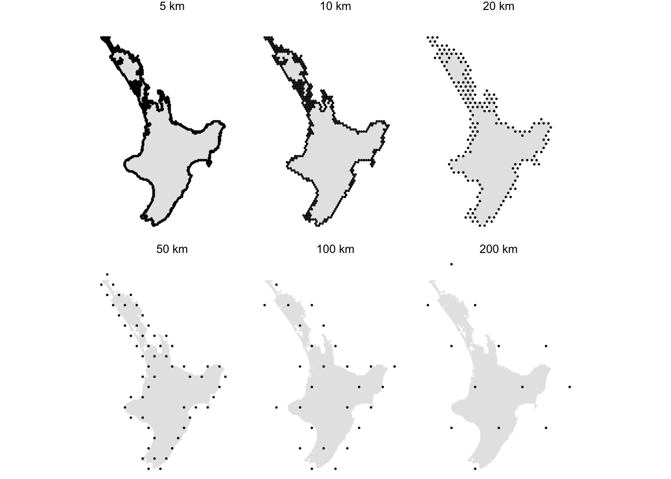

Figure 7: Map series of the hex grid centres based method.

A closing thought

This method makes me think that perhaps one way to go here might be counting discrete global grid cells along a line at a series of resolutions, although discrete global grid cells are not strictly equal in size and that might offend purists. A very cursory search suggests I am not the first person to think of this. If you are interested, see this paper:

Ghosh P. 2025. Measuring fractal dimension using discrete global grid systems. arXiv:2506.18175

It’s only been on arXiv a couple of months, so I’m not that far off the pace!

Footnotes

Nobody ever got rich writing niche textbooks so it’s no real sacrifice for us.↩︎
Geographic Information Analysis, pages 13-16.↩︎
You’ll find Robert Hijmans’ take on this here.↩︎
Such curves are important for geohashes and hierarchical indexing schemes: see this page for more.↩︎
‘Much faster’ is an understatement, even italicised.↩︎
As Dana Tomlin was wont to say, Yes raster is faster / But raster is vaster / And vector. . . / Just seems more correcter. This is one of those GIS things that is difficult to source. The attribution to Tomlin is according to Keith Clarke.↩︎