Code
library(igraph)
library(sfnetworks)
library(sf)
library(dplyr)
library(tidyr)
library(DescTools)
library(ggplot2)
library(cols4all)
library(patchwork)

set.seed(1)A just published paper1 by Marc Barthelemy and Geoff Boeing proposes an interesting new model for making synthetic urban street networks. Setting aside the slightly breathless language (‘universal’ model? really?!2) the model had me scurrying for my computer to make my own version, as these things tend to do when they (i) are interesting, and (ii) make cool pictures.
That usually means first NetLogo (it’s the tool I think with), then R (it does graphics well, even if the language itself is a bit wonky). Marc and Geoff have written their model in Python, which is probably what I would do too if my plan was to do lots of analysis. That’s not the goal here. I was just interesting in exploring the model a little. The question of what happens when you add ‘shortcuts’ to a two-dimensional graph in terms of the network structure is something I’ve explored to some degree or another since my PhD work when I used Duncan Watts’s small world rewiring method to make non-uniform 2D lattices. I returned to it at least in passing in Computing Geographically
Along the way, I changed the model a lot, probably because I’ve recently been updating the Spatial Simulation model-zoo and there are a horde of Eden growth and percolation models in that work, and those were front of mind. There’s also not a lot of point in just making the same model, right?
Although I worked out some initial ideas in NetLogo, I present the code here in R. First, as usual imports.
library(igraph)
library(sfnetworks)
library(sf)
library(dplyr)
library(tidyr)
library(DescTools)
library(ggplot2)
library(cols4all)
library(patchwork)
set.seed(1)Mostly the usual suspects, with the addition of igraph and sfneworks, and DescTools, which I must have used before because it was already in my R library, but I have no idea why. The last of these provides a simple Gini function, which I don’t use, but which is important in Marc and Geoff’s analysis, along with a function for generating all pairwise combinations of elements from a vector, a function it is surprising that base R does not offer.
Next, some functions that find repeated use in what follows.
A function for extracting the edges of a graph as a dataframe of from and to entries, along with any additional attribute data that might be associated with the edges is nice to have.
get_edge_df <- function(G) {
  df <- G |>
    as_edgelist() |>
    as.data.frame() |>
    rename(from = V1, to = V2)
  # if there are edge attributes also include those
  if (length(edge_attr_names(G)) > 0) {
    df <- df |> bind_cols(G |> edge.attributes() |> as.data.frame())
  }
  df
}Also useful is a function to add distances (i.e., edge lengths) to an edge dataset, given a table of vertices with xand y coordinate locations. This assumes that the edges dataframe has from and to attributes that correspond to the nameattribute in the vertex dataframe.
Coordinates are added by joining based on the from and to columns and used to find distances. igraph treats any edge attribute called weightas special for use in path length calculations and the like, so we give the length that name as a convenience.
add_edge_lengths <- function(edge_df, vertex_df) {
  edge_df |>
    left_join(vertex_df, by = join_by(from == name)) |>
    rename(x1 = x, y1 = y) |>
    left_join(vertex_df, by = join_by(to == name)) |>
    rename(x2 = x, y2 = y) |>
    mutate(weight = sqrt((x2 - x1) ^ 2 + (y2 - y1) ^ 2)) |>
    select(-x1, -y1, -x2, -y2)
}Only used once, but good to give them names and not clutter up the main workflow with their complicated workings are two functions that combine to collapse ‘chains’ of vertices with only two neighbours into single edges.
If we have a local formation like A—B—C3 then the goal here is to collapse that to A—C. In the paper, Marc and Geoff avoid creating vertices with two neighbours by adding two neighbours to vertices with a single neighbour. Here, because I am making the ‘background’ lattice of the network by removing edges, the problem is to to remove all such vertices. Aesthetically, as we’ll see this has the nice side-effect of introducing diagonal edges and departing a little from the strict orthogonality of the networks in the original paper.
This code was by far the most complicated piece of this to get working. Hover over the numbered circles for explanations of what’s going on at each step.
collapse_chains <- function(G) {
chains <- G |>
subgraph(V(G)[which(degree(G) == 2)]) |>
components()
vs_to_delete <- c()
es_to_add <- c()
for (i in 1:chains$no) {
vs <- names(chains$membership)[which(chains$membership == i)]
vs_to_delete <- c(vs_to_delete, vs)
ext_chain <- neighborhood(G, order = 1, nodes = vs) |>
unlist() |> names() |> unique()
end_vs <- ext_chain[which(!(ext_chain %in% vs))]
if (length(end_vs) == 2) {
es_to_add <- c(es_to_add, end_vs)
}
}
G |> add_edges(es_to_add) |>
delete_vertices(vs_to_delete) |>
largest_component() |>
simplify()
}
collapse_all_chains <- function(G) {
while (degree_distribution(G)[3] > 0) {
G <- G |> collapse_chains()
}
G
}subgraph in combination with degree to get all vertices with only two neighbors.
componentsfunction provides us with information on which of the subgraphs of vertices of degree 2 are connected to one another.
vs_to_delete and es_to_add are lists of the degree-2 vertices we will remove, and edges that will be added back in to reconnect the graph across gaps left by removing vertices.
ext_chain extends the chain of degree-2 vertices to any neighbors by one-link. The added vertices in the extended chain are the ones that may have to be reconnected.
end_vs removes the chain itself from the extended chain leaving only end points.
es_to_add list when the number of additional vertices is the usual two.
degree_distribution is the number of degree-2 vertices in the graph.
The plot.igraph function is difficult to control particularly when it comes to imposing equal aspect ratios and layering graphs in the same space on top of one another, so the somewhat ad hoc function below converts graphs to sfnetwork graphs which can be plotted by ggplot.
ggplot_graph <- function(G, plot = NULL) {
  G_sf <- sfnetwork(nodes = G |>
                      vertex.attributes() |>
                      as.data.frame() |>
                      st_as_sf(coords = c("x", "y")),
                    edges = G |> get_edge_df(),
                    directed = FALSE,
                    edges_as_lines = TRUE)
  edges <- G_sf |> activate("edges") |> st_as_sf()
  if (is.null(plot)) {
    plot <- ggplot()
    if ("betweenness" %in% names(edges)) {
      plot <- plot +
        geom_sf(data = edges, aes(colour = betweenness, linewidth = betweenness)) +
        scale_color_binned_c4a_seq(palette = "tableau.classic_red") +
        scale_linewidth(range = c(0.1, 3)) +
        guides(colour = "none", linewidth = "none")
    } else {
      plot <- plot +
        geom_sf(data = edges)
    }
  } else {
    plot <- plot +
      geom_sf(data = edges, colour = "red", linewidth = 2)
  }
  plot + theme_void()
}In this section I work through the process of creating a small network, assembling a series of functions along the way, so that at the end of this notebook it’s simple to chain them all together to make a larger ‘synthetic city network’.
First we need some very basic parameters
radius <- 10
n_mst <- 25
prop_retained <- 0.85-radius to +radius inclusive.
We start with a complete lattice, optionally trimmed to a ‘circle’. Astute observers will notice that trimming the lattice to a circle assumes that the coordinates are centred on \((0, 0)\).
get_lattice <- function(radius, circular = TRUE) {
  lims <- -radius:radius
  extent <- length(lims)
  size <- extent * extent
  lattice <- igraph::make_lattice(c(extent, extent), dim = 2) |>
    set_vertex_attr("name", value = 1:size |> as.character()) |>
    set_vertex_attr("x", value = rep(lims, extent)) |>
    set_vertex_attr("y", value = rep(lims, each = extent))
  if (circular) {
    disc <- sqrt(vertex_attr(lattice, "x") ^ 2 +
                 vertex_attr(lattice, "y") ^ 2) <= radius
    lattice <- lattice |>
      subgraph(vids = V(lattice)$name[disc])
  }
  lattice
}
lattice <- get_lattice(radius)
Having made the lattice, let’s see what it looks like.
ggplot_graph(lattice)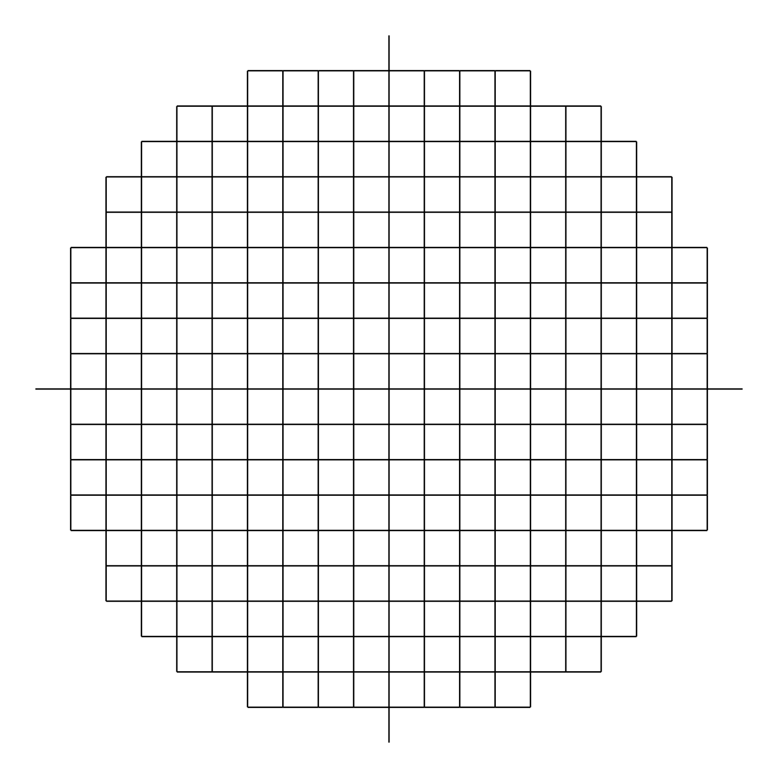
The lattice ‘thinning’ is a two stage process. First we randomly remove some edges, then we apply the degree-2 vertex collapsing process explained in the previous section.
# get the lattice edge and vertex dataframes
get_thinned_lattice <- function(G, proportion_retained) {
  vs <- G |>
    vertex.attributes() |>
    as.data.frame()
  G |>
    get_edge_df() |>
    slice_sample(prop = proportion_retained) |>
    graph_from_data_frame(directed = FALSE, vertices = vs) |>
    largest_component() |>
    collapse_all_chains() |>
    get_edge_df() |>
    add_edge_lengths(vs) |>
    graph_from_data_frame(directed = FALSE, vertices = vs) |>
    largest_component()
}
thinned_lattice <- get_thinned_lattice(lattice, prop_retained)
And again, we can see what this looks like.
plot1 <- ggplot_graph(thinned_lattice)
plot1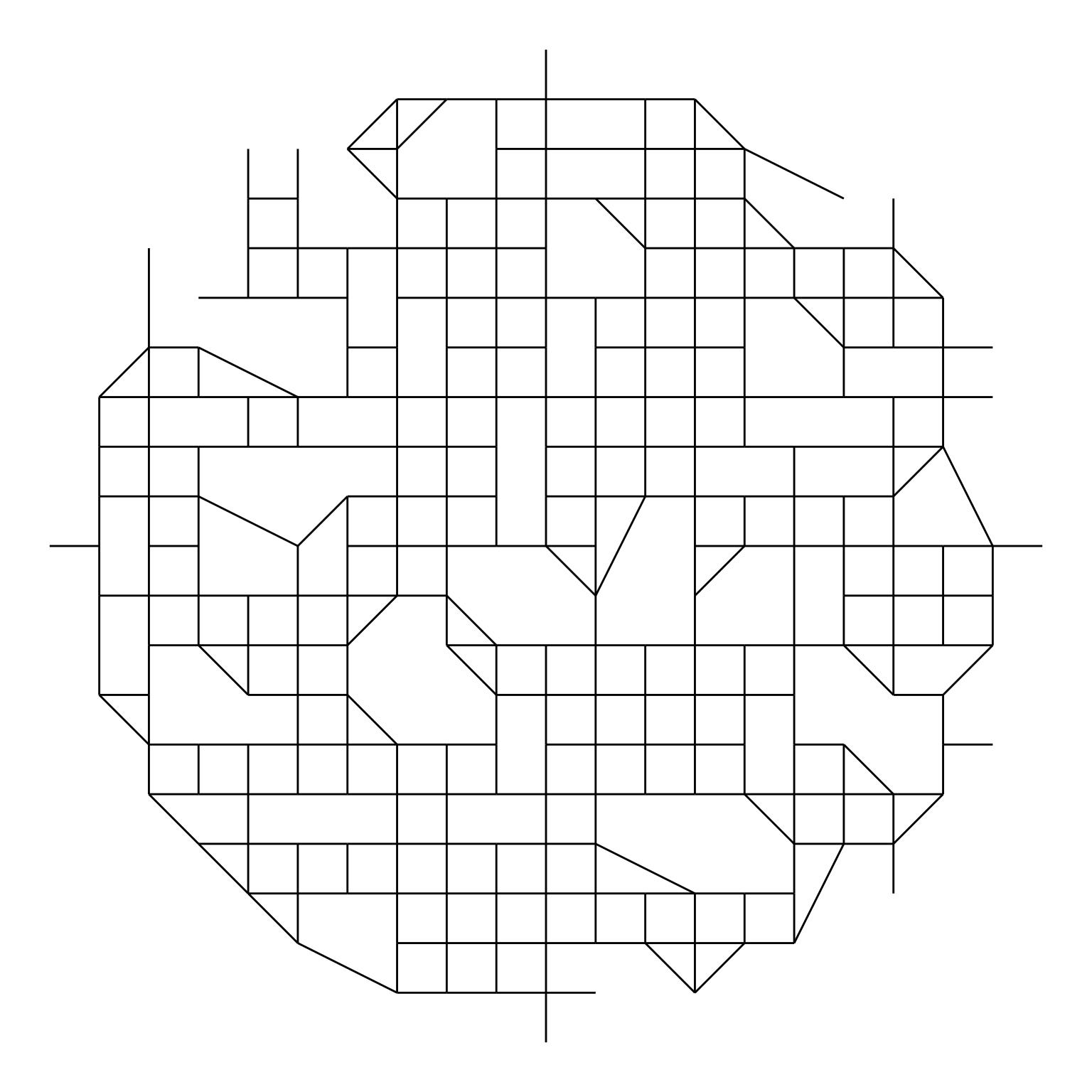
Central to the Barthelemy and Boeing model is a network backbone derived from a minimum spanning tree. As we’ll see, the current model doesn’t seem to need this backbone to yield skewed distributions of the edge betweenness centrality, but it’s easy enough to make a minimum spanning tree and add it to the thinned lattice to see its effect on the overall structure.
get_mst_from_random_subset <- function(G, n) {
  vs <- G |>
    vertex.attributes() |>
    as.data.frame()
  es <- G |>
    get_edge_df() |>
    add_edge_lengths(vs)
  mst_vs <- vs |>
    slice_sample(n = n)
  mst_all_es <- CombPairs(mst_vs$name) |>
    mutate(from = as.character(X1), to = as.character(X2)) |>
    select(-X1, -X2) |>
    add_edge_lengths(vs)
  mst_all_es |>
    graph_from_data_frame(directed = FALSE, vertices = mst_vs) %>%
    mst()
}
min_ST <- get_mst_from_random_subset(thinned_lattice, n_mst)
And we can use our nice graph plotting function to overlay this on the thinned lattice, noting that so far the two graphs are entirely separate.
plot2 <- ggplot_graph(min_ST, plot = plot1)
plot2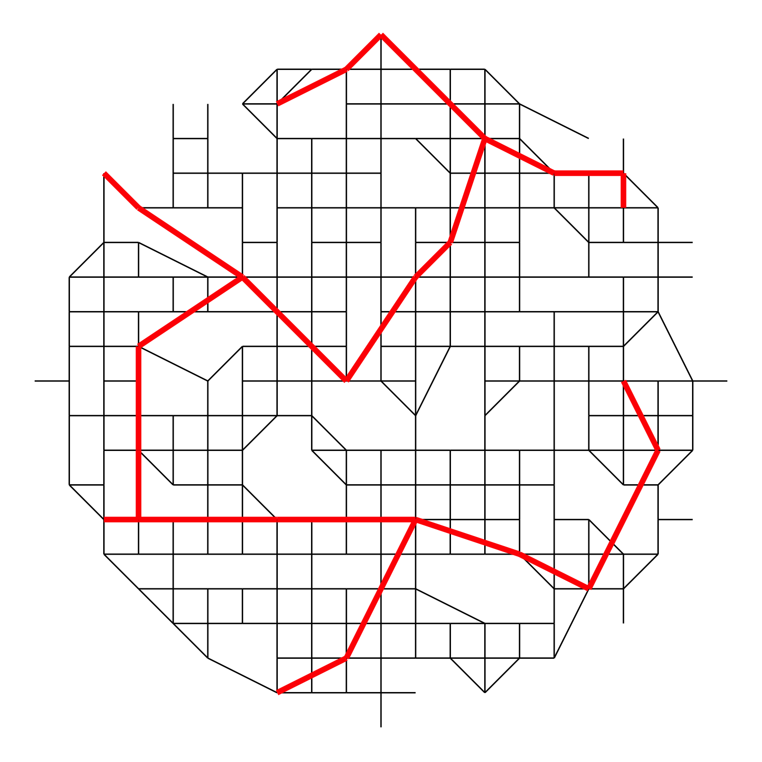
That long east-west edge in the minimum spanning tree won’t make a lot of difference in this example, because when we calculate centrality based on shortest paths (see the next section) it is based on edge weights and it doesn’t provide a shortcut. This is a lot more likely to happen in a small network like this one, but it’s an important thing to keep in mind when considering overall characteristics of this approach. The Barthelemy and Boeing model grows the lattice part of the network out from the nodes of the minimum spanning tree, so that the MST edges are necessarily shortcuts. Adding the MST to an existing lattice, in the absence of different ‘speeds’ along edges (imagine the MST was the freeway network or transit) is unlikely to make as much difference as the backbone does in their model.
OK. Here’s a betweenness centrality map of the thinned lattice without any included minimum spanning tree backbone.
eb1 <- thinned_lattice |> edge_betweenness(directed = FALSE)
thinned_lattice <- thinned_lattice |>
set_edge_attr(name = "betweenness", value = eb1)plot3 <- ggplot_graph(thinned_lattice) +
ggtitle("Thinned lattice") +
theme(plot.title = element_text(hjust = 0.5))
plot3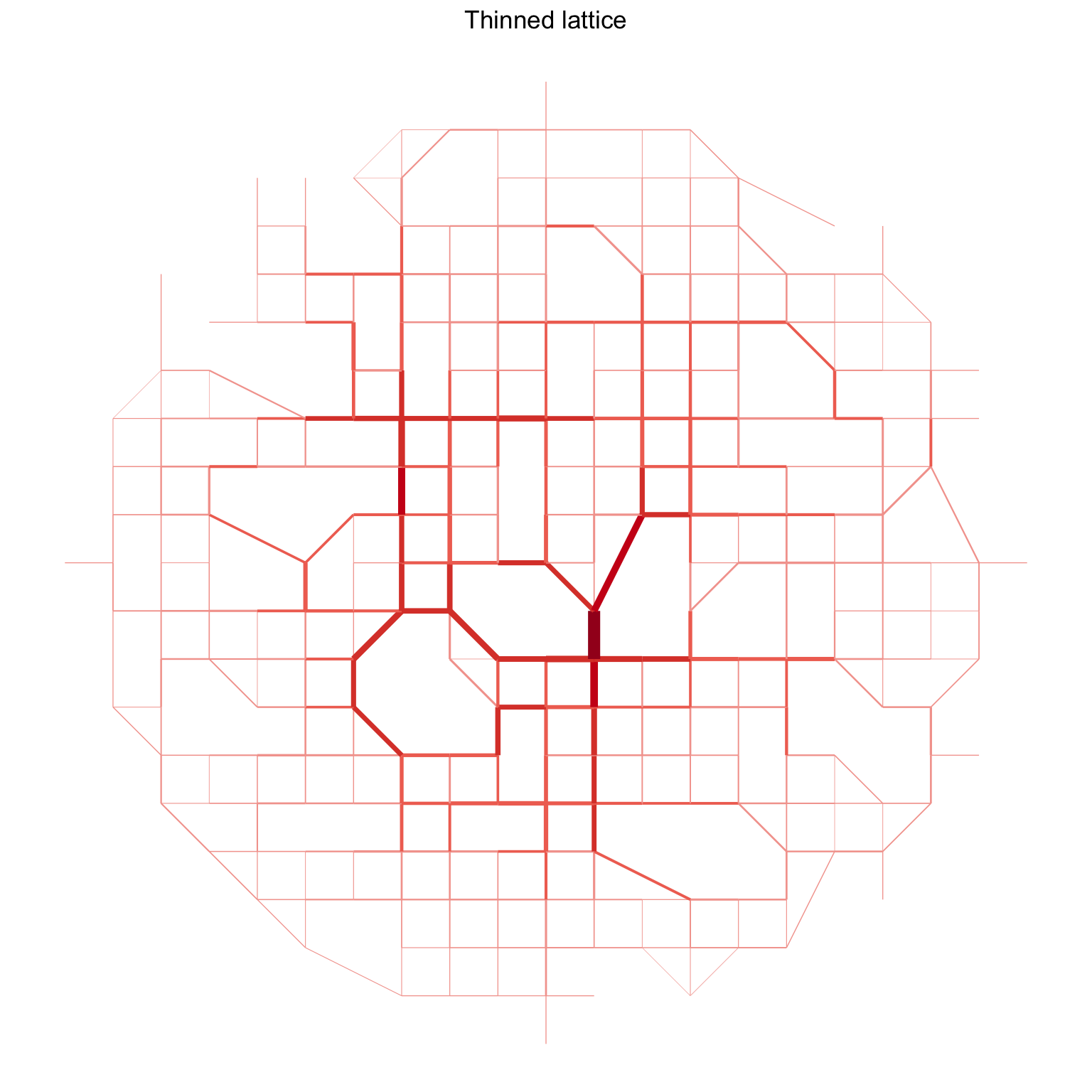
It seems like this process has resulted in a network structure that already has a fairly defined backbone of higher centrality edges. I’m not making any claims here about how congruent with empirical data on real city networks this structure is: that kind of thing is very much in Marc and Geoff’s realm of expertise. Nevertheless the structure is interesting.
Now we can add the minimum spanning tree backbone into the thinned lattice.
# merge the new edges into the existing
add_subgraph <- function(G, x) {
  vs <- G |>
    vertex.attributes() |>
    as.data.frame()
  G |> get_edge_df() |>
    bind_rows(x |> get_edge_df() |> add_edge_lengths(vs)) |>
    graph_from_data_frame(directed = FALSE, vertices = vs)
}
combined_lattice <- add_subgraph(thinned_lattice, min_ST)
eb2 <- combined_lattice |> edge_betweenness(directed = FALSE)
combined_lattice <- combined_lattice |>
  set_edge_attr(name = "betweenness", value = eb2)
And map the two networks side-by-side. For the very little that it’s worth, the distribution of betweenness centrality doesn’t appear as different as I’d have expected, going into this process. But clearly much more extensive investigation would be required before jumping to any conclusions.
plot4 <- ggplot_graph(combined_lattice) +
  ggtitle("Combined with MST") +
  theme(plot.title = element_text(hjust = 0.5))
plot3 | plot4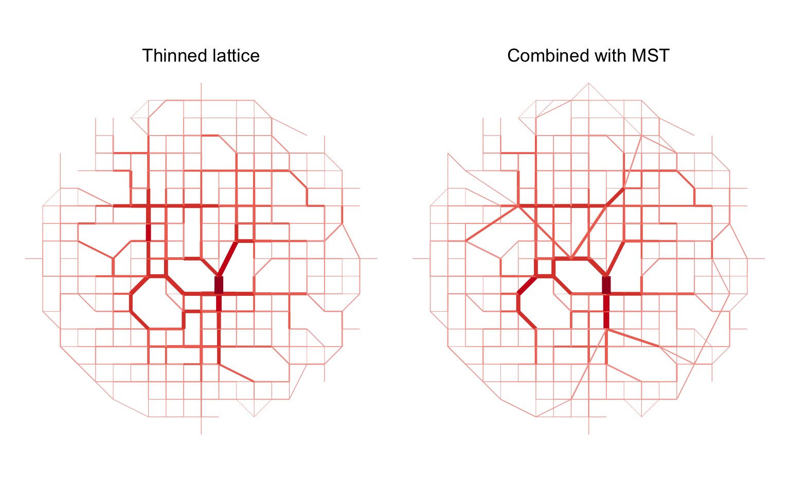
The small network shown above is really to illustrate the process step by step. In the code below, a wrapper function let’s us run everything at once and generate a bigger network in one go.
make_city <- function(radius, prop, n_mst = 0, circular = TRUE) {
  L <- get_lattice(radius, circular = circular) |>
    get_thinned_lattice(prop)
  if (n_mst > 1) {
    M <- get_mst_from_random_subset(L, n_mst)
    L <- add_subgraph(L, M)
  }
  L |> set_edge_attr(
    name = "betweenness",
    value = edge_betweenness(L, directed = FALSE)
  )
}
city <- make_city(50, 0.75, 0)
plot5 <- ggplot_graph(city)
plot5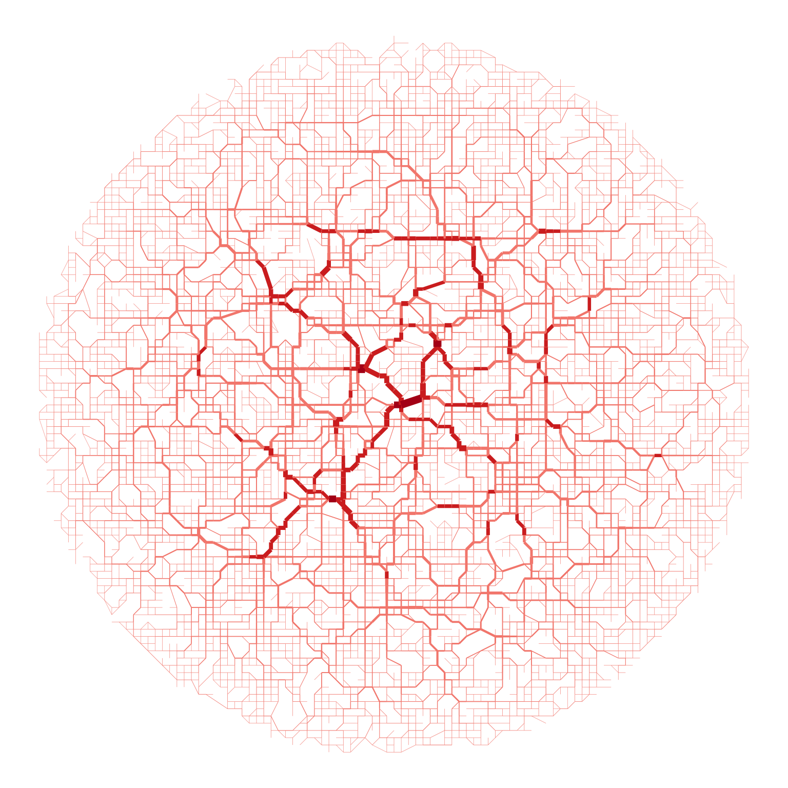
Even if this is all just a bit of messing around with network code, the pictures are satisfyingly ‘city-like’!
![]()
Barthelemy M and G Boeing. 2025. Universal Model of Urban Street Networks. Physical Review Letters 135(13): 137401.↩︎
As Geoff notes on his blog the apparently lost indefinite article in the title, which adds to the grandiosity of the claim, is apparently because the journal doesn’t allow titles to start with an indefinite article. There’s probably something fairly deep about the psyche of phyicists to learn from that rather odd rule. Saying that, it’s not clear that the notion of ‘a’ universal model is logically coherent. But I digress…↩︎
Yes, I’m using em-dashes, and I don’t care if it makes you think I am an AI.↩︎