GIS, a transformational approach

Like a few of the earlier posts on a transformational approach to GIS this one turned into a rabbit hole, and so it will only cover field→point and field→line transformations. This takes us into the realm of surface networks and the journey has given me a better appreciation of some of the reasons that this seemingly promising approach to surface analysis has never quite taken off.¹

Code

library(sf)
library(terra)
library(dplyr)
library(stringr)
library(tmap)
library(whitebox)
library(cols4all)

Before we get started, a convenience function for making binary rasters into point data sets.

Code

raster_to_points <- function(r) {
  pts <- r |> 
    as.points() |>
    st_as_sf() |>
    rename(value = 1) |>
    dplyr::filter(as.logical(value))
}

From fields…

The data this time, perhaps a little ambitiously are a digital elevation model of the area around the Zealandia wildlife sanctuary in Wellington. This is an area of about 225 hectares surrounded by a predator proof fence that keeps out the various mammalian critters that have been so devastating to Aotearoa’s birdlife providing those birds with an opportunity to get established and thrive. In combination with local predator trapping efforts Zealandia has seen very encouraging signs of recovery in local native bird populations. Even in the few years we have been in Wellington the uptick in the numbers of kākā in particular has been obvious as a result of ‘spillover’ from the sanctuary into nearby suburbs. So much so that from time to time kākā are on the verge of becoming a pest.²

Code

dem <- rast("zealandia-5m.tif")
tracks <- st_read("tracks.gpkg") |> select(highway)
fence <- st_read("fences.gpkg") |> select(NAME, TYPE) |> filter(TYPE == "Main")
streams <- st_read("streams.gpkg") |> select()
lake <- st_read("lake.gpkg") |> select(name)
roads <- st_read("roads.gpkg") |> select(name, highway)
hillshade <- shade(terrain(dem, unit = "radians"), 
                   terrain(dem, v = "aspect", unit = "radians"), 
                   angle = 30, direction = 135)

Anyway, here’s a map. The focus of this post is on the underlying DEM which characteristically for Wellington is rugged!

Code

tm_shape(dem) +
  tm_raster(
    col.scale = tm_scale_continuous(values = "hcl.terrain2", 
                                    limits = c(50, 400)),
    col.legend = tm_legend_hide()) +
  tm_shape(hillshade) +
  tm_raster(
    col.scale = tm_scale_continuous(values = "brewer.greys"),
    col_alpha = 0.25, col.legend = tm_legend_hide()) +
  tm_shape(fence) +
  tm_lines(col = "purple", lwd = 4) +
  tm_shape(tracks) +
  tm_lines(lwd = 1, lty = "dashed") +
  tm_shape(streams) +
  tm_lines(col = "dodgerblue") +
  tm_shape(roads) +
  tm_lines(col = "black", lwd = 2.5) +
  tm_lines(col = "white", lwd =1.5) +
  tm_shape(lake) +
  tm_fill(fill = "dodgerblue") +
  tm_scalebar(position = c(0.01, 0.04), text.size = .75,
              bg = TRUE, bg.color = "white", bg.alpha = 0.5)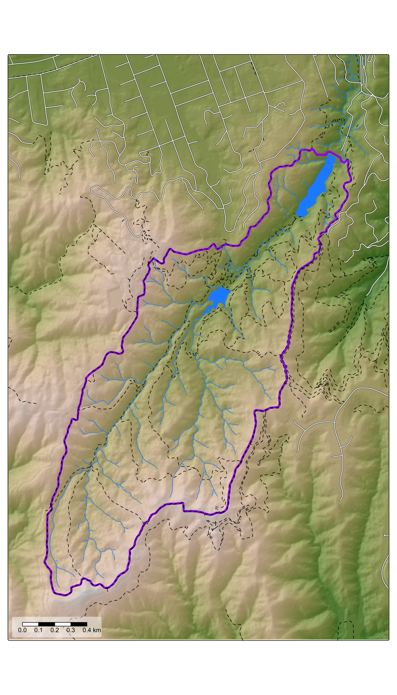

Figure 1: General map of the Zealandia sanctuary showing predator proof fence (purple), tracks (dashed lines), and surrounding urban streets.

OK, on to the code (such as it is).

… To points

Surface specific points to be more precise. According to an early computer cartography text

Surface-specific points have a higher information content than surface random-points. Surface-specific points, however, exhibit a hierarchy among themselves. These points are, in decreasing order, peaks and pits, passes, and ridge and course lines. These features not only tell their values, but also give some idea about their surroundings. In the environs of a peak, we can say that everything else will be lower (Peucker 1972³, page 29)

We can find pits using a built in function in terra that operates on a flow direction surface,⁴ but we can also find pits and peaks directly with simple focal operations on the DEM.

Code

pits <- dem |>
  focal(w = 3, function(x) all(x[5] < x[-5])) |>
  raster_to_points()

peaks <- dem |>
  focal(w = 3, function(x) all(x[5] > x[-5])) |>
  raster_to_points()

If we combine these into a single point data set and tag them as pit or peak

Code

pts <- bind_rows(
  pits |> mutate(type = "pit"),
  peaks |> mutate(type = "peak")
)

then we can see them on our original surface:

Code

tm_shape(dem) +
  tm_raster(
    col.scale = tm_scale_continuous(values = "brewer.greys"),
    col.legend = tm_legend_hide()) +
  tm_shape(streams) +
  tm_lines(col = "dodgerblue") +
  tm_shape(pts) +
  tm_dots(fill = "type",
    fill.scale = tm_scale_categorical(values = "brewer.set1"),
    fill.legend = tm_legend_hide())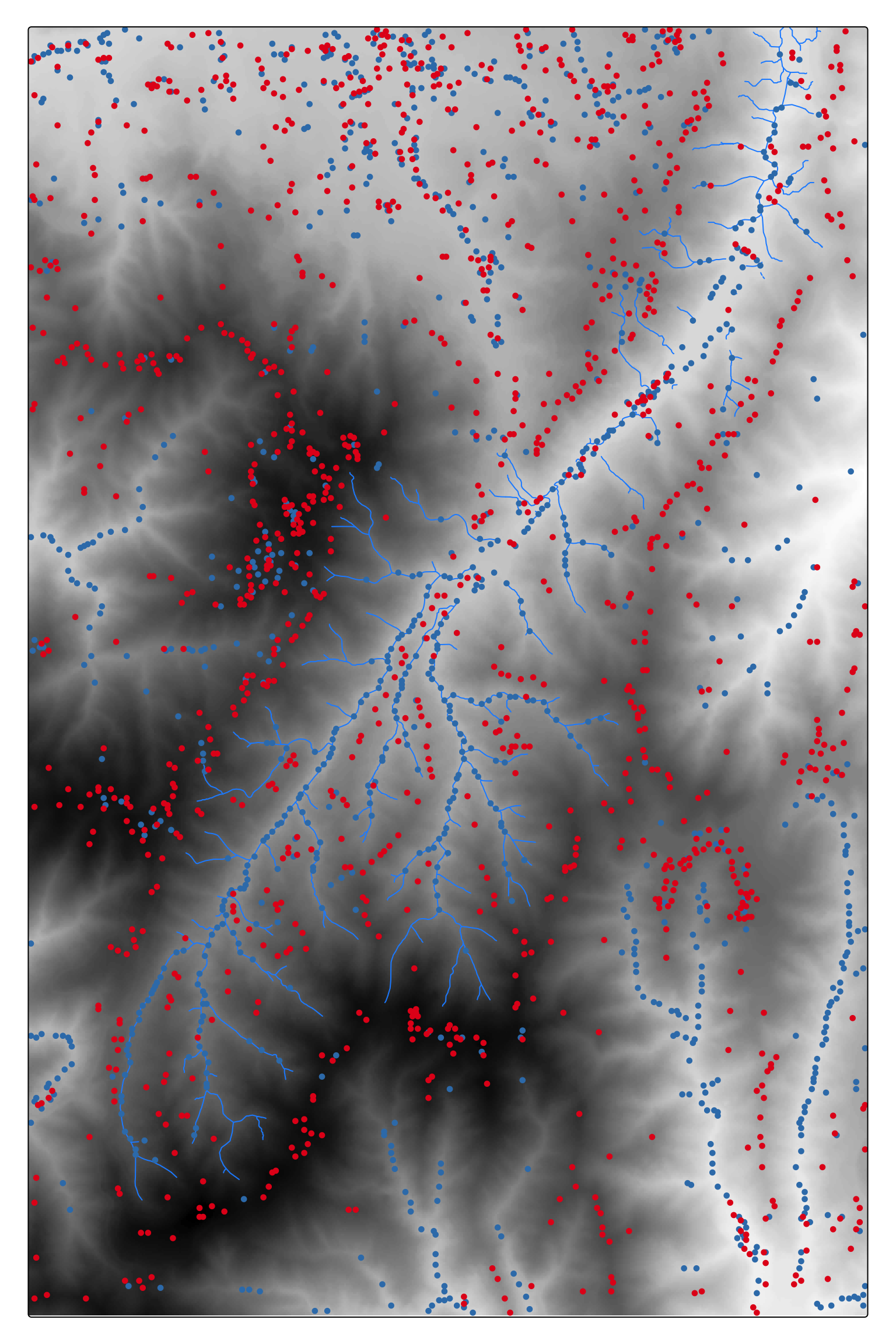

Figure 2: Pits (blue) and peaks (red) on the original DEM surface

It’s easy to see that pits are generally found in valleys and peaks on ridge lines. We can get further reassurance on this by mapping the peaks and pits relative to the surface’s geomorphons⁵ using the Whitebox Tools whitebox::wbt_geomorphons() function.

Code

geomorphon_labels <- read.csv("geomorphons.csv") |>
  pull(Landform.Type) |>
  as.vector()
wbt_geomorphons(dem, "geomorphons.tif", search = 3, threshold = 0)
geomorphons <- rast("geomorphons.tif") |>
  subst(1:10, geomorphon_labels) 
geomorphons_cropped <- geomorphons |>
  crop(ext(ext(geomorphons) + c(-15, -15)))

Overlaying our pits and peaks on the geomorphon map confirms that the locations of pits and peaks are where we would expect to find them. Here and elsewhere click on the map for a closer look.

Code

tm_shape(geomorphons_cropped) +
  tm_raster(
    col.scale = tm_scale_categorical(
      levels = geomorphon_labels, 
      values = c(c4a_na("brewer.rd_bu"), c4a("brewer.rd_bu", n = 9))),
    col.legend = tm_legend(
      title = "", orientation = "landscape", 
      item.height = 1.5, item.width = 4)) +
  tm_shape(pts) +
  tm_dots(shape = "type", size = 0.5,
    shape.scale = tm_scale_categorical(values = c(2, 6)),
    shape.legend = tm_legend_hide()) +
  tm_layout(
    legend.frame.lwd = 0,
    legend.width = 55,
    legend.position = tm_pos_out(
      cell.h = "center", cell.v = "bottom", pos.h = "center"))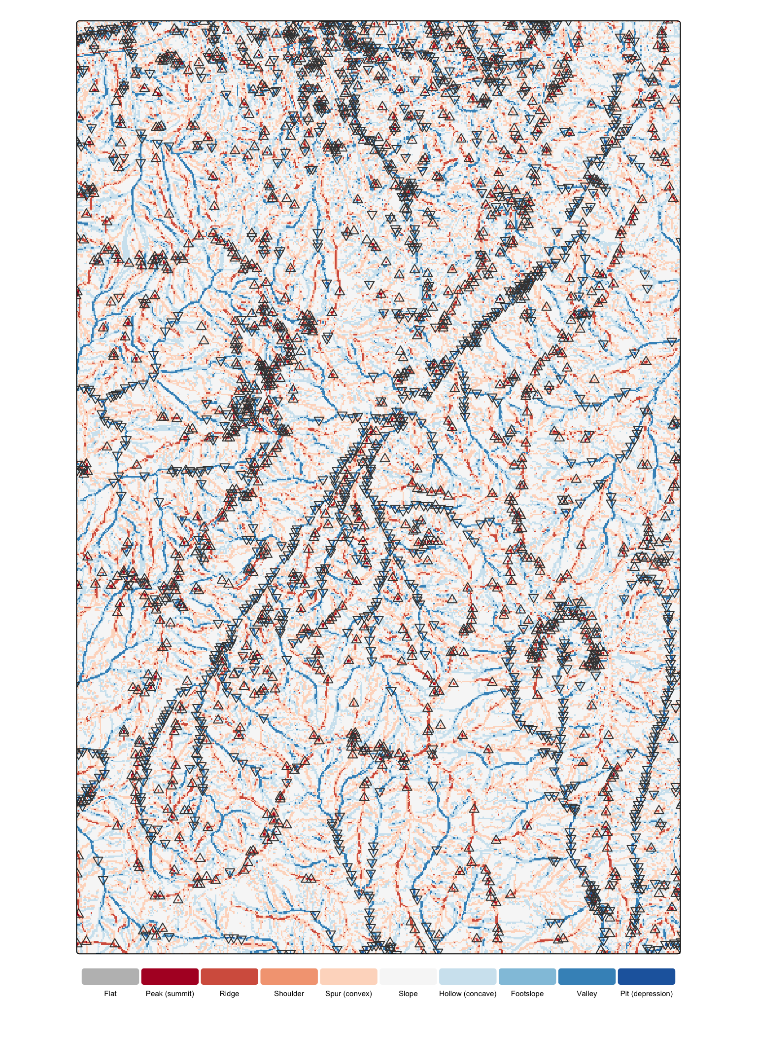

Figure 3: Geomorphons detected by whitebox tools with peaks (up point triangles) and pits (down pointing triangles)

Passes (saddle points)

The other surface-specific points that are of interest are passes or saddle points. These have zero slope, but opposite signed curvature in (at least) two directions. By contrast, pits and peaks have the same signed curvature in all directions. Passes are trickier to identify than pits and peaks.

I’ve written some code to do this in a crude fashion below, although as we’ll see shortly there is much more thorough prior work on this, which we will use in the next section.

Code

count_sign_flips <- function(m) {
  bdy_indices <- c(1, 2, 3, 6, 9, 8, 7, 4, 1)
  sum(c(m)[bdy_indices[1:8]] * c(m)[bdy_indices[2:9]] < 0)
}

is_pass <- function(m) {
  count_sign_flips(m) %in% c(4, 6, 8)
}

passes <- dem |> 
  focal(w = 3, function(x) is_pass(x[5] - x)) |>
  raster_to_points() |>
  mutate(type = "pass")

The is_pass() function first determines how many times the sign flips as we go around the outer elements in a 3-by-3 matrix of height differences between those outer elements and the focal element in the matrix. Then, if the number of sign flips is 4, 6, or 8, the location is tagged as a pass.

And here is the output:

Code

tm_shape(geomorphons_cropped) +
  tm_raster(
    col.scale = tm_scale_categorical(
      levels = geomorphon_labels, 
      values = c(c4a_na("brewer.rd_bu"), c4a("brewer.rd_bu", n = 9))),
    col.legend = tm_legend(
      title = "", orientation = "landscape", 
      item.height = 1.5, item.width = 4)) +
  tm_shape(passes) +
  tm_dots(shape = 1, size = 0.35) +
  tm_layout(
    legend.frame.lwd = 0,
    legend.width = 55,
    legend.position = tm_pos_out(
      cell.h = "center", cell.v = "bottom", pos.h = "center"))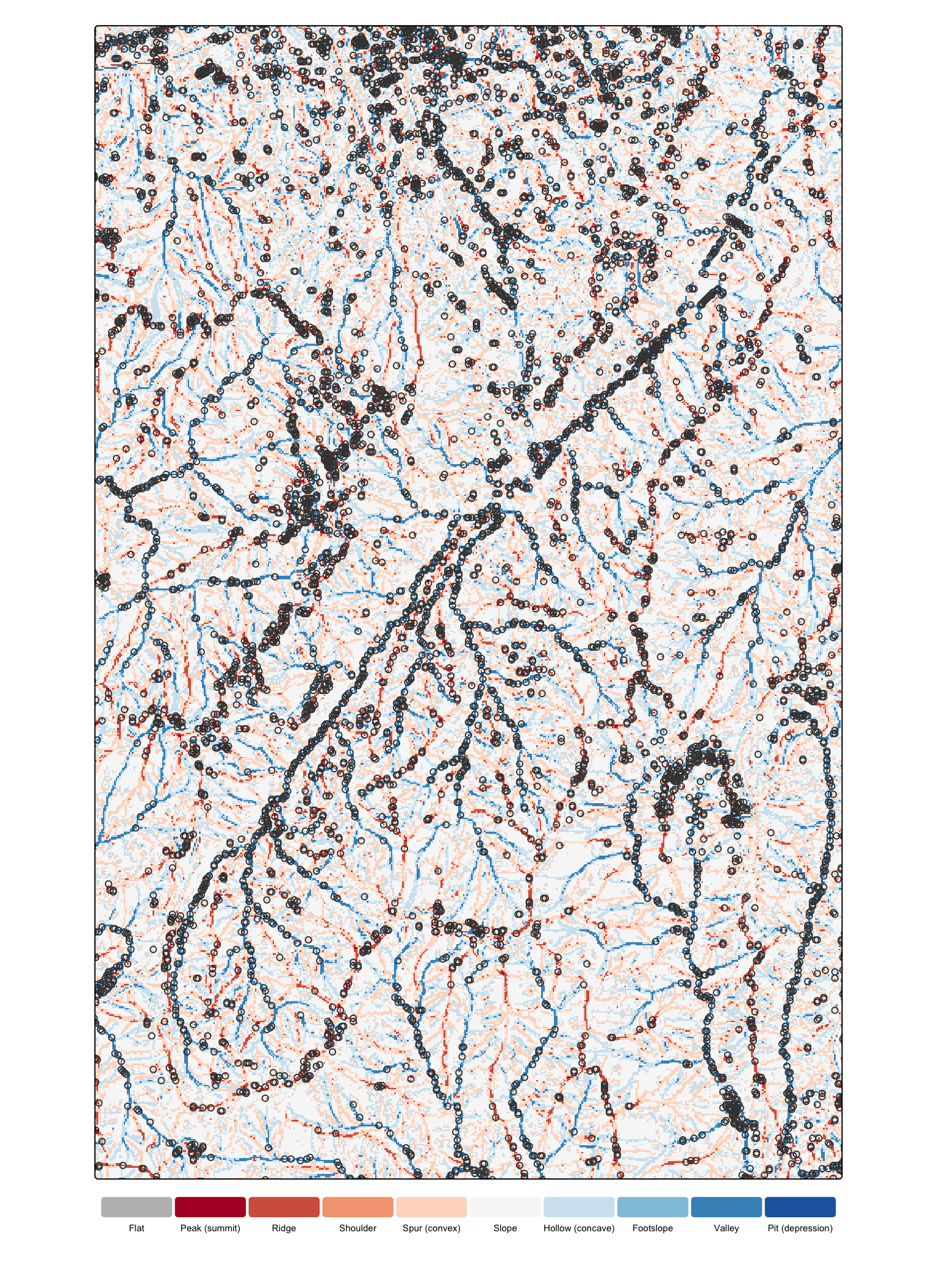

Figure 4: Passes mapped on top of geomorphons

I should emphasise that the above is not production code, not by a long shot. I know for a fact that it sometimes counts an odd number of sign flips, which should never happen (think about it). It also doesn’t handle situations where the height difference between a cell and one of its eight neighbours is zero. These facts are related. Smarter code would allow (as the geomorphon method does) for a ternary classification of the relationship between a cell and its neighbours (higher, lower, and almost level with), but as we’ll see in just a paragraph or three, this problem has already been addressed by somebody else, so… moving on.

… To lines

OK… so why did we go to all the trouble of finding passes (however inadequately)? Thereby hangs a tale. We can use these three types of surface-specific point to construct a topological representation of a surface known as a surface network, and that is the designated output for field to line transformations in that pesky table on page 26 of Geographic Information Analysis.

Topological considerations tell us that a well-formed surface should be such that peaks, pits, and passes form a tripartite network with peaks connected to passes via ridges, and passes to pits via courses (or much better via thalwegs), and with no direct links between peaks and pits.⁶

Work on surface networks in giscience in spite of its very early first appearances is spotty. Gerd Wolf, a leading researcher on the topic, writes—I think a little regretfully—about how the approach has been adopted in other fields.⁷ Wolf himself proposed a method for cartographic generalisation of surfaces using the information contained in surface networks (essentially by preserving their ridge and thalweg structure) as far back as 1988.⁸

The most recent work I’ve found on the topic is by Eric Guilbert and colleagues (Guilbert 2021⁹, Guilbert et al. 2023¹⁰) and hallelujah! there is runnable code that produces well-formed surface networks.

An important part of this code is finding the right number of passes. This is because the topological constraints imply that

\[ n_{\mathrm{pass}} - n_{\mathrm{pit}} - n_{\mathrm{peak}} = 2 \]

and the kinds of issues noted in the previous section in relation to my crude pass detection function are tricky to avoid due to the approximate nature of raster surface representations. The papers linked in the footnotes go into some detail on how these issues can be resolved, but in essence it revolves around introducing the right number of diagonal connections between cells in the grid to maximise the number of saddle points detected.

Anyhow, all that is by the by. As noted, there is runnable python code available. I ran it on the Zealandia DEM data¹¹ and here’s the result.

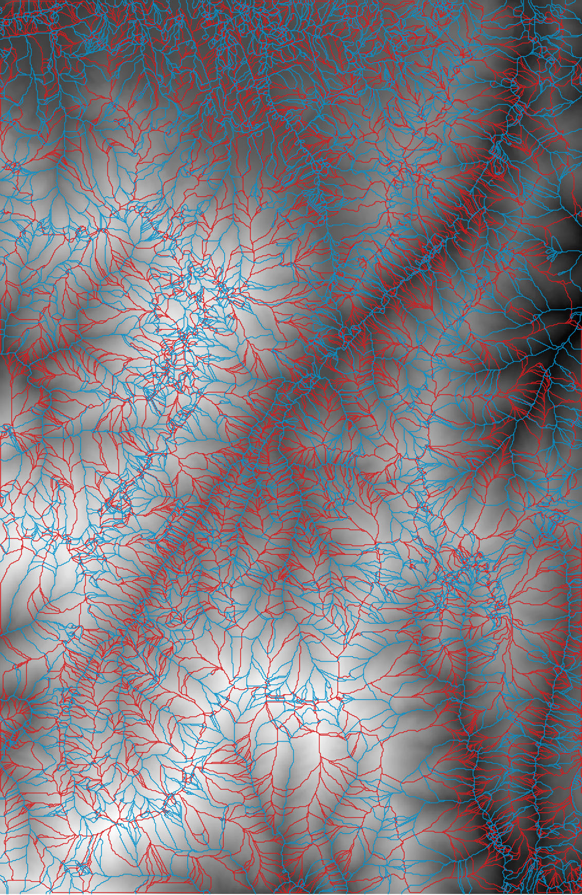
Figure 5: The surface network generated by Eric Guilbert’s python code for the Zealandia study area, showing ridges (red) and thalwegs (blue)

The surface network representation allows the terrain to be partitioned into hills (regions surrounded by thalwegs) and dales (regions surrounded by ridges). Terrain faces with two thalweg and two ridge sides, and a sequence of corners pit-pass-peak-pass can also be identified. The latest work by Eric Guilbert and colleagues looks to me like it goes a long way to putting surface networks into useful relation with more established methods of terrain analysis that tend to emphasise (understandably so) the identification of hydrological networks.

A pause for breath

Have I mentioned before how outrageously cheeky is the casual suggestion that you see how many of these transformations you can accomplish,

[i]f you already know enough to navigate your way around a GIS (Geographic Information Analysis, page 26)

My belated apologies to anyone traumatised by taking this suggestion literally. Indeed these posts on a transformational approach to GIS have been an interesting exercise in discovering how preposterous that throwaway remark really is.

On a more positive note, surface networks deserve more attention than they’ve gotten from the community over the decades, but their reliable construction has proved elusive. Perhaps now that there is at least one tool out there that is up to the task they’ll make their way into the mainstream and beginner would-be geospatial analysts won’t be left wondering why they can’t construct a surface network in spite of already knowing enough to navigate their way around a GIS.

Next up, and closing out this series will be field→area and field→field transformations.

Footnotes

TL;DR; data problems make constructing surface networks challenging.↩︎
We worry for our gutters from time to time—those beaks are powerful.↩︎
Peucker T. Computer Cartography. Resource Paper No. 17, College Geography Commission, Association of American Geographers, 1972↩︎
And by inverting the surface we can also find peaks.↩︎
See Jasiewicz J and TF Stepinski. 2013. Geomorphons — a pattern recognition approach to classification and mapping of landforms. Geomorphology 182 147–156.↩︎
Pfaltz JL. 1976. Surface networks. Geographical Analysis 8(1) 77-93.↩︎
Wolf GW. 2014. Knowledge diffusion from GIScience to other fields: the example of the usage of weighted surface networks in nanotechnology. International Journal of Geographical Information Science 28(7) 1401-1424.↩︎
Wolf GW. 1988. Weighted surface networks and their application to cartographic generalization. In W Barth (ed) Visualisierungstechniken und Algorithmen. Informatik-Fachberichte, 182. Springer, Berlin, Heidelberg. If you’re really keen complete FORTRAN code is available in this paper: Wolf GW. 1991. A FORTRAN subroutine for cartographic generalization. Computers & Geosciences 17(10) 1359-1381.↩︎
Guilbert E. 2021. Surface network extraction from high resolution digital terrain models. Journal of Spatial Information Science 22 33-59↩︎
Guilbert E, F Lessard, N Perreault, and S Jutras. 2023. Surface network and drainagenetwork: towards a common datastructure Journal of Spatial Information Science 26 53-77↩︎
I’m not crazy: I tried it first on something much simpler.↩︎