Code
# package imports
library(sf)
library(rmapshaper)
library(terra)
library(dplyr)
library(ggplot2)
library(cols4all)I did all of the 30 Day Map Challenge in 2023 and I won’t be repeating that experience again in a hurry. Last year I skipped it completely. This year I’ll do a few here and there as the mood takes me, especially if as in this example, I already have a lot of the material to hand.
Unlike some of the more ‘tutorial’ posts on the website, I’ll leave the explanations to the code comments, and just get on with making the map.
# package imports
library(sf)
library(rmapshaper)
library(terra)
library(dplyr)
library(ggplot2)
library(cols4all)The map that got me thinking I could do ‘lines’ quickly was a vector field ‘hachure map’ of a DEM, which you’ll find here where the lines representing the gradient of a DEM were centred on the raster cells. Work by others on hachures1 suggests that it’s better to position the hachures along contour lines.
First a couple of convenience functions.
# round x to nearest y
round_to_nearest <- function(x, y) round(x / y) * y

# get contour levels for supplied dem at specified interval
contour_levels <- function(dem, interval) {
  range_z <- range(values(dem)) |> round_to_nearest(interval)
  seq(range_z[1], range_z[2], interval)
}
These support a function to get points at equal intervals along contour lines from a DEM specified by spacing on contours contour_interval apart.
get_contour_pts <- function(dem, spacing = 10, contour_interval = 5) {
contour_lines <- dem |>
as.contour(levels = contour_levels(dem, contour_interval)) |>
st_as_sf() |>
ms_explode() |>
mutate(length = st_length(geometry) |> units::drop_units())
lines <- contour_lines |> pull(geometry) |> lapply(st_sfc)
line_lengths <- contour_lines |> pull(length)
mapply(st_line_interpolate,
lines,
mapply(seq, 0, line_lengths, spacing)) |>
do.call(what = c) |>
data.frame() |>
st_sf(crs = 2193)
}st_cast("LINESTRING") here it discards all but the first line in each MULTILINESTRING. rmapshaper::explode() does what I want, which is to break the MULTILINESTRINGs into individual LINESTRINGs.
mapply here, but it’s too much fun not to. The outer one applies st_line_interpolate to the linestrings, and the inner one makes sequences of steps at the required spacing along each contour.
c) to convert to a points dataframe.
The next function takes a set of points, and assigns slope, aspect, and hillshade values from rasters to them to return a dataframe with all the information needed to make hachures (at least for my purposes).
get_geomorph_df <- function(pts, slope, aspect, hillshade) {
dx <- sin(aspect) * tan(slope)
names(dx) <- "dx"
dy <- cos(aspect) * tan(slope)
names(dy) <- "dy"
pts |>
st_coordinates() |>
data.frame() |>
rename(x = X, y = Y) |>
bind_cols(extract(slope, pts, ID = FALSE)) |>
bind_cols(extract(dx, pts, ID = FALSE)) |>
bind_cols(extract(dy, pts, ID = FALSE)) |>
bind_cols(extract(hillshade, pts, ID = FALSE))
}The function below takes the data compiled by the previous function and assembles line segments to be used as hachures. It scales the hachures to a length specified by the scale argument, starting from the contour and running uphill. I found this orientation gave me nicer results on this terrain than running them downhill from the contours. The function could be modified to displace the hachures in relation to the contour lines, perhaps starting a little uphill and extending downhill across them without too much difficulty.2 In one version of this code, I had that option, but it was too many things to think about, so in the end I left it out.3
get_hachure_vectors <- function(df, scale = 25) {
df |> mutate(x0 = x, x1 = x - dx * scale,
y0 = y, y1 = y - dy * scale) |>
select(x0, x1, y0, y1) |>
apply(1, matrix, ncol = 2, simplify = FALSE) |>
lapply(st_linestring) |>
st_sfc() |>
as.data.frame() |>
st_sf(crs = 2193) |>
bind_cols(df)
}(x0 y0) to (x1 y1) pairs.
First we read in and process the DEM.
dem <- rast("zealandia-5m.tif")
cellsize <- res(dem)[1]
# this DEM has a row of NAs so get rid of them
dem <- dem |> crop(ext(dem) + c(0, 0, -cellsize, 0))
gauss <- focalMat(dem, 4, "Gauss")
dem <- dem |> focal(gauss, mean, expand = TRUE)
slope <- dem |> terrain(unit = "radians")
aspect <- dem |> terrain(v = "aspect", unit = "radians")
hillshade <- shade(slope, aspect, direction = 135, normalize = TRUE)
dem <- dem |> crop(ext(dem) + rep(-cellsize, 4))
slope <- slope |> crop(dem)
aspect <- aspect |> crop(dem)
hillshade <- hillshade |> crop(dem)
cxy <- dem |>
ext() |>
matrix(ncol = 2) |>
apply(2, mean)And now we can run the functions from above to get a set of hachures. I’ve experimented with settings, and a contour interval of 5m with points at 10m spacing along them is quite nice for this DEM.
points <- get_contour_pts(dem, spacing = 10, contour_interval = 5)
points |> head()
Simple feature collection with 6 features and 0 fields
Geometry type: POINT
Dimension: XY
Bounding box: xmin: 1747094 ymin: 5426809 xmax: 1747096 ymax: 5426857
Projected CRS: NZGD2000 / New Zealand Transverse Mercator 2000
geometry
1 POINT (1747096 5426809)
2 POINT (1747095 5426819)
3 POINT (1747095 5426829)
4 POINT (1747095 5426839)
5 POINT (1747094 5426849)
6 POINT (1747095 5426857)Next make the geomorphometric data.
df <- get_geomorph_df(points, slope, aspect, hillshade)
df |> glimpse()
Rows: 79,646
Columns: 6
$ x <dbl> 1747096, 1747095, 1747095, 1747095, 1747094, 1747095, 174709…
$ y <dbl> 5426809, 5426819, 5426829, 5426839, 5426849, 5426857, 542678…
$ slope <dbl> 0.07065191, 0.35487763, 0.36189409, 0.37607592, 0.31732243, …
$ dx <dbl> 0.04492523, 0.36862739, 0.37601937, 0.39448706, 0.31067836, …
$ dy <dbl> 0.054681579, 0.037854596, -0.043843913, -0.017379723, 0.1064…
$ hillshade <dbl> 178.62155, 208.62245, 218.69818, 216.55379, 196.04494, 205.8…And form hachures.
hachures <- get_hachure_vectors(df, 20)
hachures |> glimpse()
Rows: 79,646
Columns: 7
$ x <dbl> 1747096, 1747095, 1747095, 1747095, 1747094, 1747095, 174709…
$ y <dbl> 5426809, 5426819, 5426829, 5426839, 5426849, 5426857, 542678…
$ slope <dbl> 0.07065191, 0.35487763, 0.36189409, 0.37607592, 0.31732243, …
$ dx <dbl> 0.04492523, 0.36862739, 0.37601937, 0.39448706, 0.31067836, …
$ dy <dbl> 0.054681579, 0.037854596, -0.043843913, -0.017379723, 0.1064…
$ hillshade <dbl> 178.62155, 208.62245, 218.69818, 216.55379, 196.04494, 205.8…
$ geometry <LINESTRING [m]> LINESTRING (1747096 5426809..., LINESTRING (17470…Here’s a map of a 1km square part of the area showing the relation of the hachures to the contour lines.
ggplot() +
  geom_sf(
    data = as.contour(dem, levels = contour_levels(dem, 5)) |> st_as_sf(),
    aes(colour = level), linewidth = 1) +
  scale_colour_continuous_c4a_seq(
    palette = "-tableau.green_gold", limits = c(50, 500)) +
  geom_sf(data = hachures) +
  coord_sf(xlim = cxy[1] + c(-500, 500),
           ylim = cxy[2] + c(-500, 500), expand = FALSE) +
  guides(colour = "none") +
  theme_void()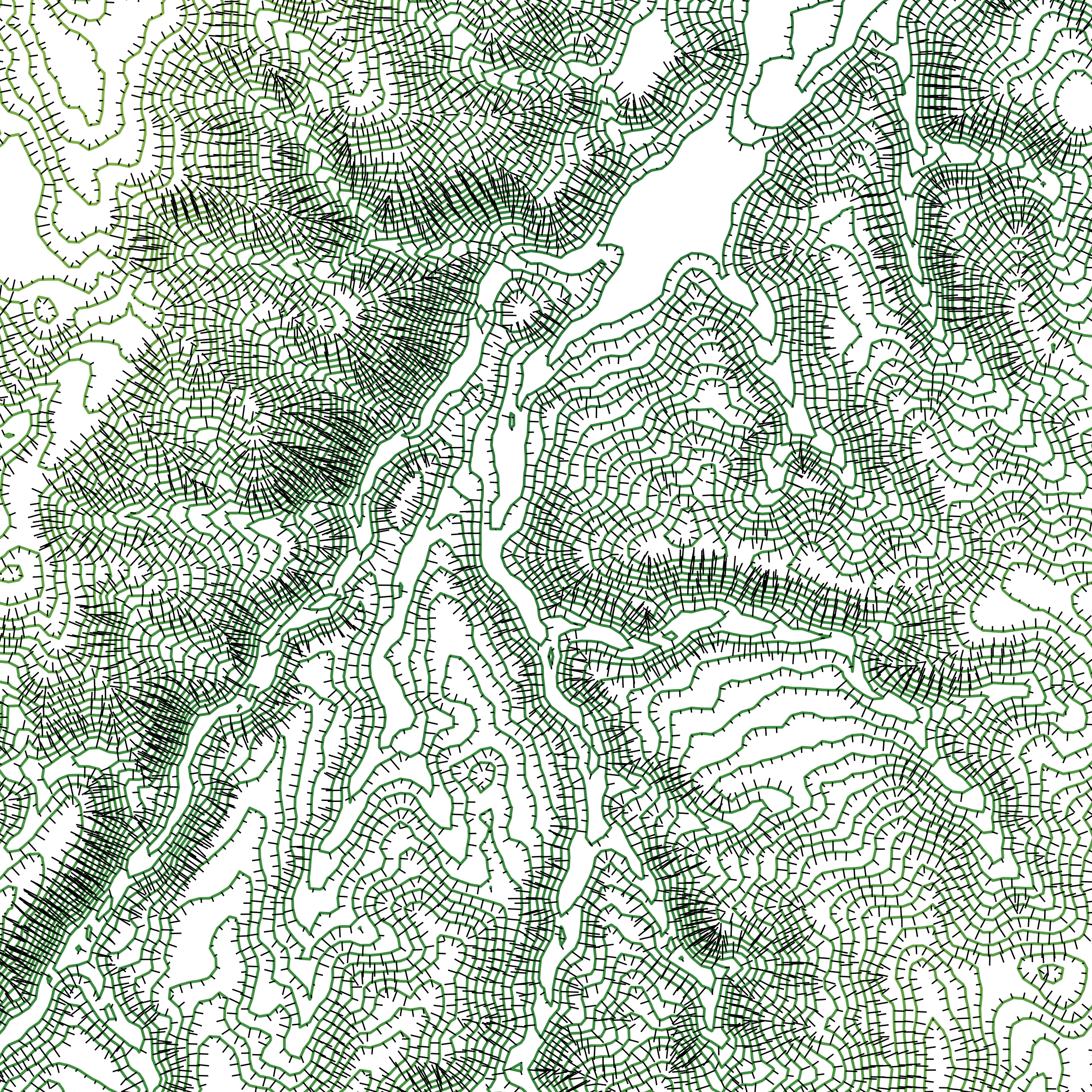
Here’s a final (R-generated) map, using the hillshade attribute to lighten or darken the hachures based on that attribute of the data, and making the line thickness of hachures dependent on the slope. I’ve added streams and lakes to show that the hachures ‘make sense’.
ggplot() +
  geom_sf(data = hachures, aes(linewidth = slope ^ 2, colour = sqrt(hillshade))) +
  scale_linewidth_identity() +
  scale_colour_distiller(palette = "Greys", direction = 1) +
  geom_sf(data = lake, fill = "skyblue", colour = NA) +
  geom_sf(data = streams, colour = "dodgerblue", linewidth = 0.5) +
  guides(colour = "none", linewidth = "none") +
  coord_sf(xlim = ext(dem)[1:2], ylim = ext(dem)[3:4], expand = FALSE) +
  theme_void()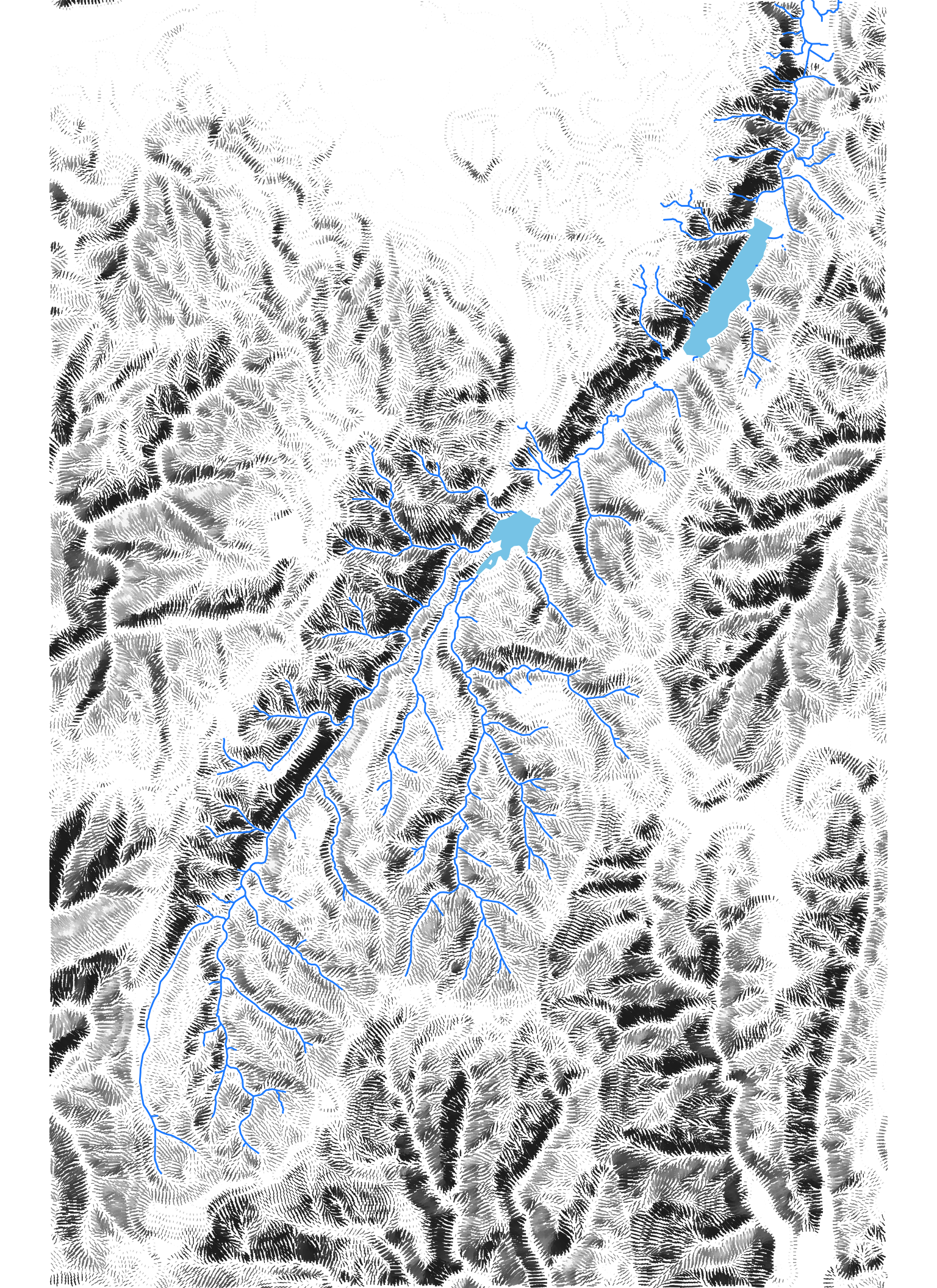
By exporting the data to points, and working with geometry generators in QGIS we can make hachures that are elongated triangles, so that the hachures are thicker at their lower elevation ends.
Here’s a map I made that way.
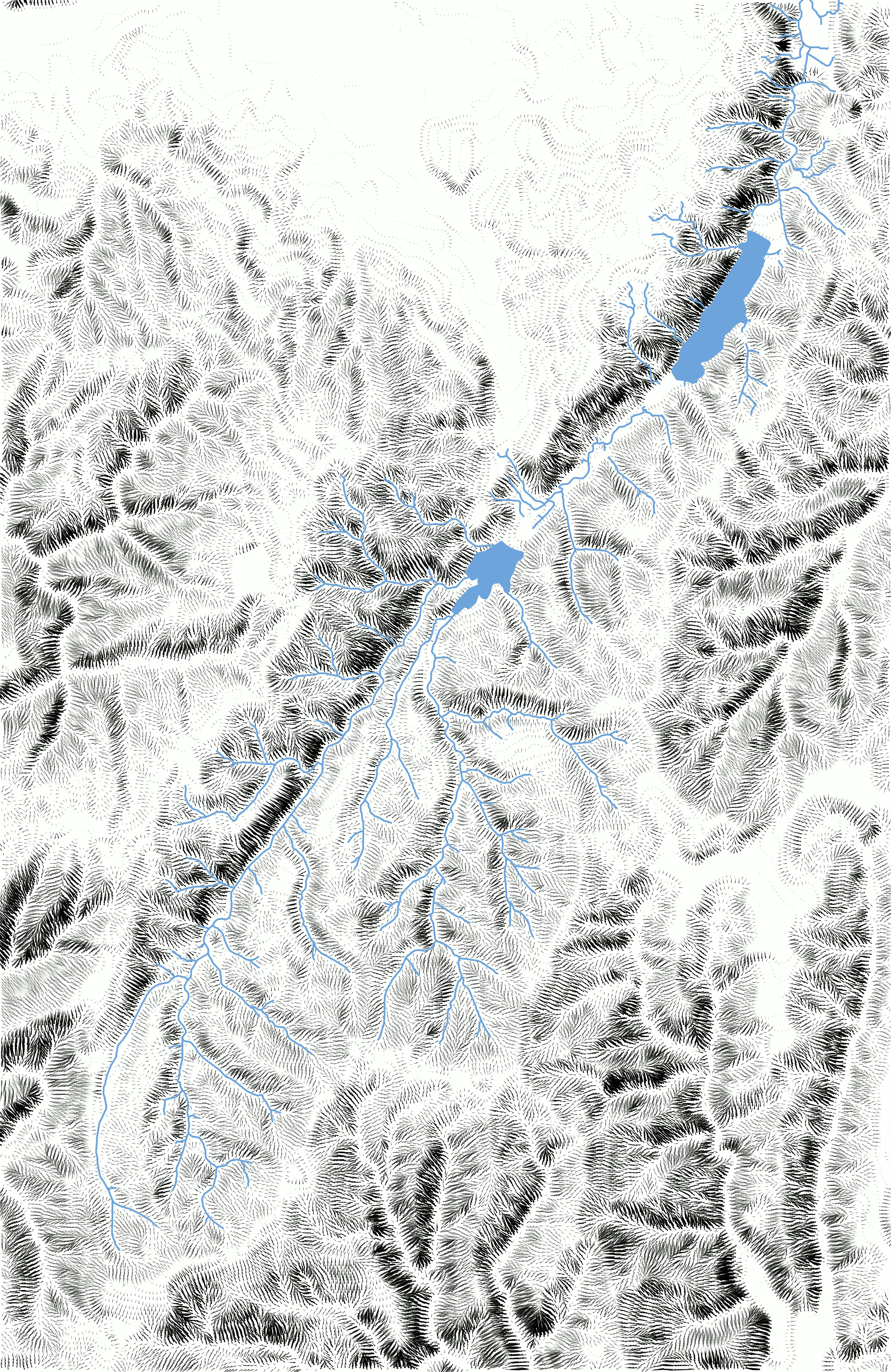
If you zoom in (click on the image) you’ll see that the hachures are elongated triangles. I don’t know if that means they are still ‘lines’ or not.4 I tried to get this effect using the ggarrow and ggquiver packages, but the former was memory-limited and slow for data this size, and the latter is not flexible enough.
This used the following geometry generator expression to generate polygon geometries:
make_triangle(
    make_point($x - 25 * "dx", $y - 25 * "dy"),
    make_point($x - 2 * "dy", $y + 2 * "dx"),
    make_point($x + 2 * "dy", $y - 2 * "dx")
)
and the following expression for the colour fill
color_rgba(
    0, 0, 0,
    255 * sqrt(scale_linear("hillshade", 0, 255, 0, 1))
)
A more complete hachure map solution would require that we consider relationships between the hachures and other features (streams, lakes, etc.). The kind of thing a cartographer would do, in fact.
Overall this took a bit more work to refine the map from the rough cut of a few days ago than I hoped, but I’m reasonably happy with this version, even as it leaves plenty of scope for improvement.
![]()