30 Day Map Challenge 2025

On Day 3 of this year’s 30 Day Map Challenge Sam Keast posted a nice Tanaka illuminated contours map, which he made in Arc loosely follow a John Nelson video.

In a comment I mentioned how much I’ve always loved this method of terrain representation ever since encountering it during my Masters in Glasgow back in 1996-7. I liked it so much that I leaned into it hard for one coursework assignment to make a tourist promotional map of a chosen location. Donegal being very much our go-to family holiday spot I chose the area around Sheephaven Bay and the Rosguill Peninsula for my subject matter. That meant that I had to manually digitise contours from a 1:50,000 topographic map of the area, and then mock up illuminated contours in CorelDraw. The map seems now to have been lost, although I dimly remember seeing it the last time we moved house, but can’t right now locate it. Never mind, if you want to know why my efforts didn’t score especially well see below.

That was a long time ago, and I’m glad to say things have got a lot easier…

library(sf)
library(terra)
library(dplyr)
library(stars)
library(ggplot2)
library(cols4all)
library(patchwork)

About Tanaka’s illuminated contours

In short, illuminated contours are an elegant way of combining contours and hillshading to represent surfaces.

The method was proposed in a paper by Kitirô Tanaka in 1950.¹ Terrain is considered to be lit (as in a hillshaded map) from some direction. The idea is to draw contours on a grey (or other mid-tone) background with black lines on dark slopes facing away from the light source, and white lines on illuminated slopes.

Line thickness is also varied with the aspect of the slope relative to the light source. Thick white lines are used on slopes facing directly towards the illumination, and thick black lines on slopes facing directly away from the light source, line thickness narrowing as slopes progressively turn to lie parallel to the direction of illumination. An example for a simple circular contour is seen in the next section if this is unclear.

When this idea was proposed, it required a steady hand. Tanaka noted that, “One may reasonably doubt whether such seemingly complicated contour lines can be easily and quickly drawn”, before going on to reassure readers that

A simple and exact method is available […]. If the tip of a drawing pen […] is filed down so that its thickness is the maximum thickness required in a contour line, and if […] the pen-point edge is kept at a fixed orientation […] parallel to the assumed horizontal direction of the incident light, then the thickness of the contour line will vary with the cosine of the angle \(\theta\). (1950, page 449)

I would venture to suggest that this was much harder to do than it was to describe! I spent some time in my Masters study using ink pens to make maps by hand, and it was an exacting business even to reliably render lines of uniform thickness, never mind varying them in a consistent way as proposed for this technique. The technical challenge goes a long way to explaining why the method has remained relatively rarely used until recently.

A crude DIY implementation

Fortunately for the unsteady of hand we can now easily approximate Tanaka’s method.

To illustrate my approach, I’ve made a single circular contour, and two copies, one offset southeast, and the other offset northwest.

circle <- st_point(c(0, 0)) |> 
  st_sfc() |> 
  data.frame() |>
  st_as_sf(crs = 2193) |>
  st_buffer(1000)
  
circle_se <- circle |> 
  mutate(geometry = geometry + c(50, -50)) |>
  st_set_crs(st_crs(circle))
  
circle_nw <- circle |> 
  mutate(geometry = geometry + c(-50, 50)) |>
  st_set_crs(st_crs(circle))

Now, layer them on top of one another southeast, centred, and northwest, in that order, coloured black, grey, and white, respectively.

ggplot() +
  geom_sf(data = circle_se, fill = "black", colour = NA) +
  geom_sf(data = circle_nw, fill = "white", colour = NA) +
  geom_sf(data = circle, fill = "grey", colour = NA) +
  theme_void() +
  theme(panel.background = element_rect(fill = "darkgrey", colour = NA))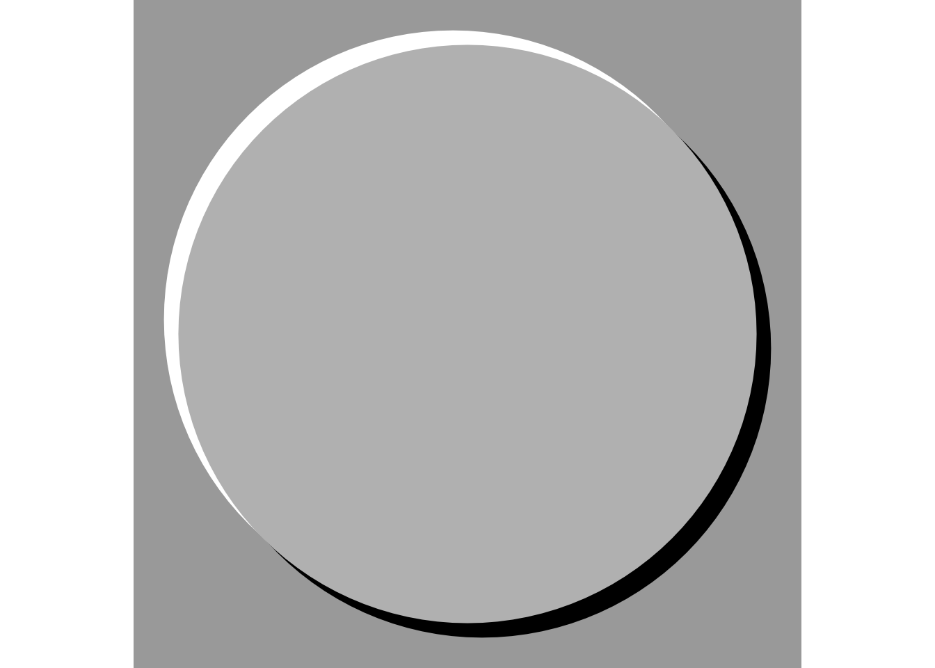

Figure 1: A single illuminated contour showing the principle behing the method: this contour is illuminated from the northwest

The effect is striking and in this crude implementation not at all hard to code. I say crude not because this approach is inaccurate but because more recent work has suggested further refinements of the method such that either the colour or thickness of contour lines varies with their facing towards the light source.² In terms of Tanaka’s original suggestion my simple approach produces lines of the correct thickness, in this fixed case for a light source from the northwest.

Assembling some reusable code

With the basis of an approach established we can assemble some functions to produce Tanaka contoured maps.

First, it’s convenient to generate from a DEM a set of evenly spaced contour levels, and given those levels to use stars::st_contour to get contour polygons.

# label: functions-to-get-polygons
round_to_nearest <- function(x, y) round(x / y) * y

contour_levels <- function(dem, interval) {
  range_z <- range(values(dem), na.rm = TRUE) |> round_to_nearest(interval)
  seq(range_z[1]- interval, range_z[2] + interval, interval)
}

get_contour_polygons <- function(dem, levels) {
  dem |> 
    st_as_stars() |> 
    st_contour(breaks = levels) |>
    st_as_sf()
}

Next a function to shift supplied contour polygons by some x and y offsets. This uses the constantly surprising functionality in sf where you can simply add a vector to the geometry attribute of an sf dataframe.

offset_shapes <- function(shapes, dx, dy) {
  shapes |>
    mutate(geometry = geometry + c(dx, dy)) |>
    st_set_crs(st_crs(shapes))
}

Next we need some code to render the various layers in the right order starting at the bottom of the stack of contour polygons, and at each level going through them in a consistent order.

The addition of layer and group attributes to the data enables the rendering order to be controlled. ggplot renders data by group, in the order that elements appear in the table, so we use arrange to sort in ascending order of Min (the elevation) and layer. We also assign all the data to a single group group = 0, and include that as an aesthetic in the call to ggplot, so that the data table sort order rendering isn’t overridden by grouping on the layer attribute.

my_tanaka_contours <- function(dem, interval, thickness, direction = 135,
                               colour = "grey", light = "white", dark = "black") {
  levels <- contour_levels(dem, interval)
  contours <- get_contour_polygons(dem, levels) |> 
    mutate(layer = 3)
  angle <- direction * pi / 180
  dx <- cos(angle) * thickness
  dy <- sin(angle) * thickness
  contours_light <- contours |> 
    offset_shapes(dx, dy) |> 
    mutate(layer = 2)
  contours_dark <- contours |> 
    offset_shapes(-dx, -dy) |> 
    mutate(layer = 1)
  all_contours <- bind_rows(contours, contours_light, contours_dark) |>
    mutate(layer = ordered(layer, levels = 1:3), group = 0) |>
    arrange(Min, layer)
  ggplot(all_contours) +
    geom_sf(aes(fill = layer, group = group), colour = NA) +
    scale_fill_manual(values = c(dark, light, colour)) +
    guides(fill = "none") +
    coord_sf(expand = FALSE) + 
    theme_void()
}

Data from Mars

Since I’m smuggling this in under the guise of Day 18 ‘Out of this world’, we need some out of this world data, so I found some Mars surface topography. Specifically, this dataset which is a high resolution digital elevation model of a crater,³ derived from Mars Reconnaissance Orbiter data by a team at the University of Arizona.

dem_raw <- rast("https://astrogeo-ard.s3-us-west-2.amazonaws.com/mars/mro/hirise/controlled/dtm/ESP_050125_1480_ESP_050046_1480/DTEED_050125_1480_050046_1480_G01.tif")

The raw data is in an equirectangular cylindrical coordinate reference system, which means it’s stretched east-west because just like on Earth meridians converge toward the poles, so we should reproject to something conformal or at least more sensible local to the area of interest. Mercator gets a lot of stick, but this is local data so it’s fine. The key thing here is to specify a spheroid that is Mars-sized, hence +R=3396190. I am also aggregating the data five-fold because at ~2 meter resolution it’s more detailed than we need (and some smoothing does no harm for this method.

proj <- "+proj=merc +lat_0=-31.46 +lon_0=-22.9 +k=1 +R=3396190 +units=m"
dem <- dem_raw |> 
  project(proj) |>
  terra::aggregate(5)
names(dem) <- "z"

And so to a couple of maps. I’ve tried one using the default grey-black-white colouring, and a second using a more Martian colour scheme.

g1 <- my_tanaka_contours(dem, 20, 20)
g2 <- my_tanaka_contours(dem, 20, 20, colour = "#ff9020",
                         light = "#f8e078", dark = "#B04030")
g1 | g2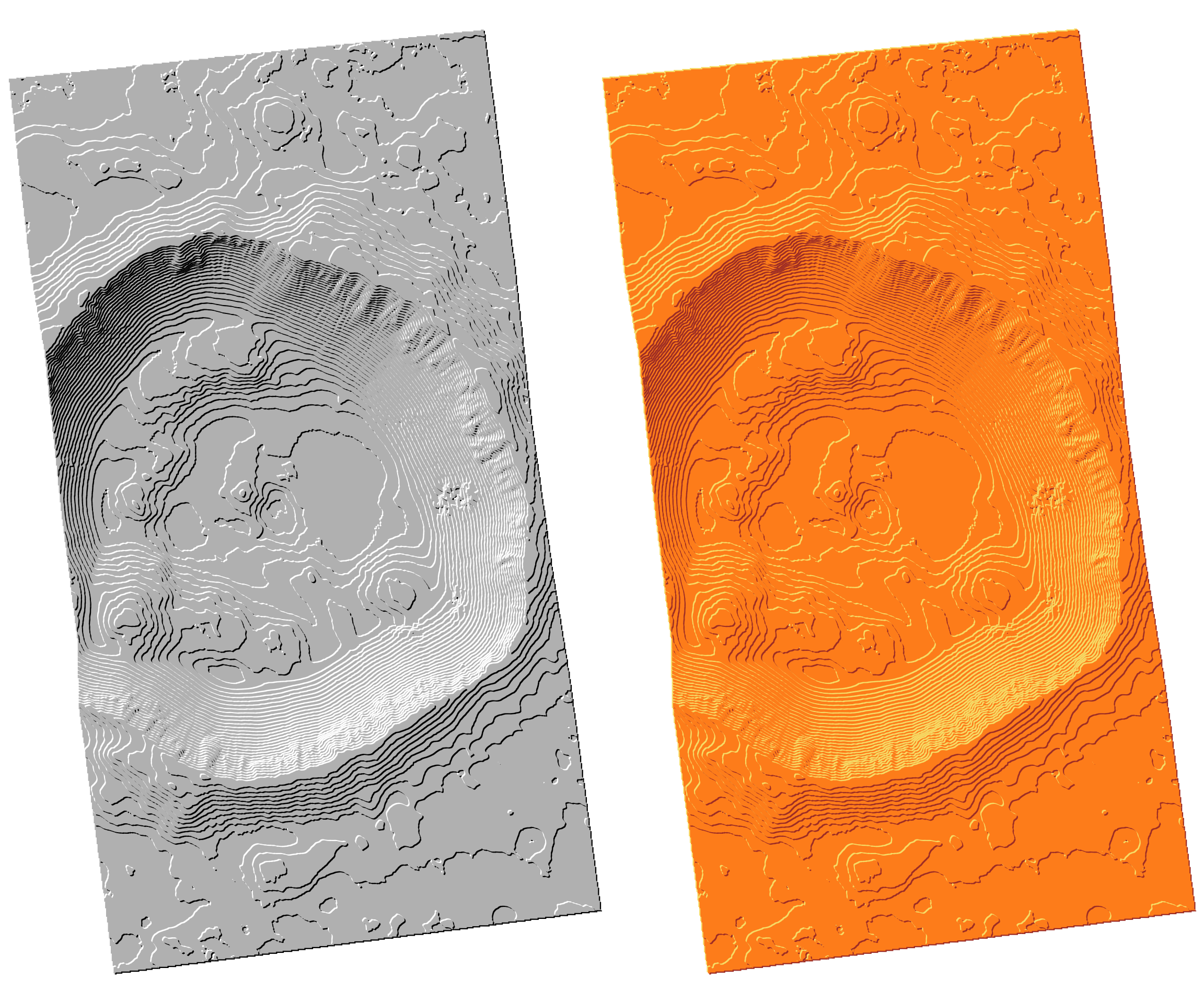

Figure 2: Two Mars crater maps using illuminated contours, one of them (perhaps) in more Mars-appropriate colours

There’s a package for that

I didn’t follow my own advice here and went ahead and wrote my own code before checking if there was already an R package out there that does Tanaka contours. Of course there is.⁴ In fact, there are two, metR and tanaka. Because the former sticks with ggplot2 style plotting I show it here.

library(metR)

dem_xy <- dem |>
  as.data.frame(xy = TRUE)

ggplot(dem_xy) + 
  geom_raster(aes(x = x, y = y), fill = "grey") +
  geom_contour_tanaka(
    aes(x = x, y = y, z = z),
    binwidth = 20, sun.angle = 45) + 
  coord_equal() + 
  theme_void()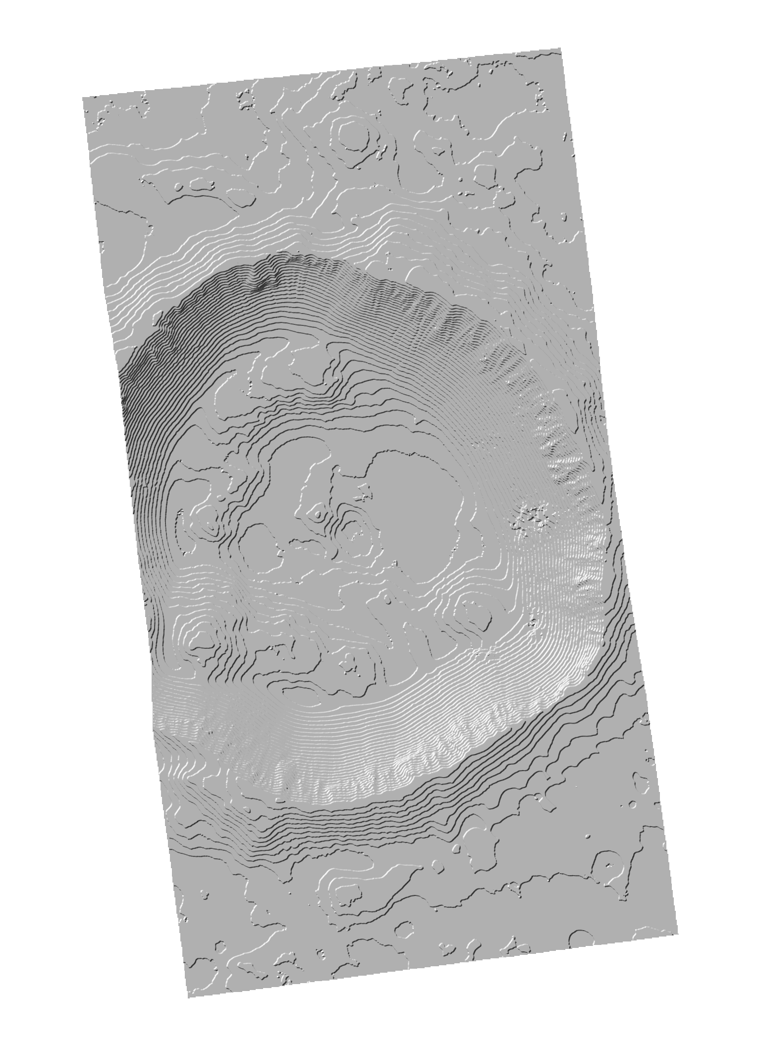 

Figure 3: A basic Tanaka contour map using metR

What’s nice about this package is that I can also colour the contours using a hypsometric colour ramp. After some experimentation (see the commented out alternatives), I decided the hcl.heat2 ramp was the most ‘Martian-looking’.

ggplot(dem_xy) + 
  geom_raster(aes(x = x, y = y, fill = z)) +
  scale_fill_continuous_c4a_seq(palette = "hcl.heat2") +
  # scale_fill_continuous_c4a_seq(palette = "hcl.terrain2") +
  # scale_fill_continuous_c4a_seq(palette = "-tableau.orange") +
  # scale_fill_continuous_c4a_seq(palette = "met.greek") +
  guides(fill = "none") +
  geom_contour_tanaka(
    aes(x = x, y = y, z = z), 
    binwidth = 20, sun.angle = 45) + 
  coord_equal() + 
  theme_void()

Figure 4: A Tanaka contour map using metR with the contour intervals hypsometrcally coloured

The tanaka package functions can also do this, although the API in that case is less clean.

For old time’s sake…

… in about one-hundredth of the time it took way back when, I thought I’d’ revisit the map from my Masters coursework, or at least the terrain representation part of it.

So I grabbed a relevant portion of the Continental Europe DTM from OpenTopography⁵ and ran it through metR’s geom_contour_tanaka.

The colours I’ve used are from memory and I know my choices were rather bold. Keep in mind that I also had to overlay symbology, placenames, and so on. It was also supposed to be a promotional map, not a tasteful topographic map. Even so, I think I went a bit overboard.

donegal <- rast("sheephaven.tif") |>
  as.data.frame(xy = TRUE)

ggplot(donegal) +
  geom_raster(aes(x = x, y = y), fill = "#209030") +
  geom_contour_tanaka(aes(x = x, y = y, z = donegal), binwidth = 50,
                      sun.angle = 45) +
  coord_sf(expand = FALSE) +
  theme_void() +
  theme(panel.background = element_rect(fill = "#3090e0"))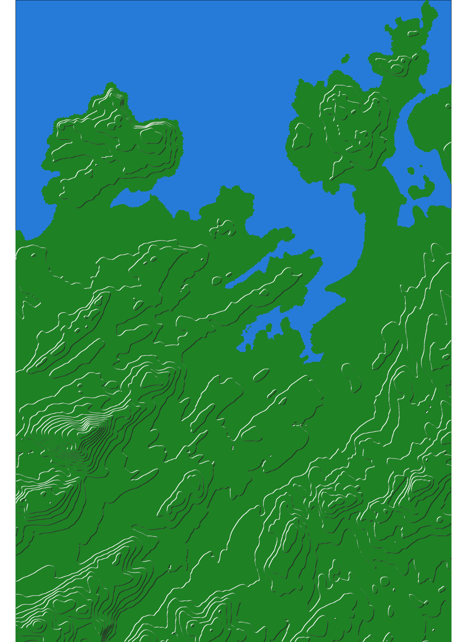

Figure 5: A mock up of the terrain elements of that tourism map of Donegal

The challenge of illuminated contours is finding a base colour that allows both the light and dark contours to show up well, and I recall experimenting endlessly with that in this design, every time having to print it out to figure out if it was working or not.

I can’t help but wonder if I’d been able to hypsometrically tint my contours back in 1996 if I’d have done a bit better on that coursework assignment.

ggplot(donegal) +
  geom_raster(aes(x = x, y = y, fill = donegal)) +
  scale_fill_continuous_c4a_seq(palette = "hcl.terrain2") +
  guides(fill = "none") +
  geom_contour_tanaka(aes(x = x, y = y, z = donegal), binwidth = 50,
                      sun.angle = 45) +
  coord_sf(expand = FALSE) +
  theme_void() +
  theme(panel.background = element_rect(fill = "#3090e0"))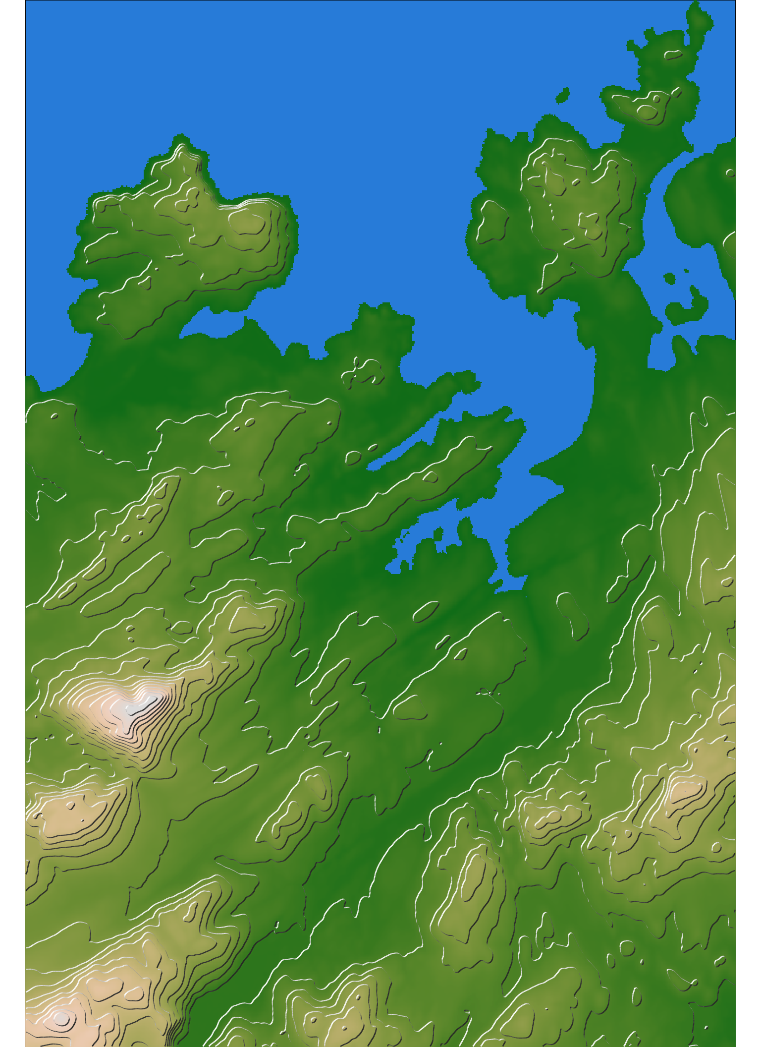

Figure 6: This time with terrain colours

Footnotes

1. Tanaka K. 1950. The relief contour method of representing topography on maps. Geographical Review 40(3) 444-456.

2. Kenelly P and AJ Kimerling. 2001. Modifications of Tanaka’s illuminated contour method. _Cartography and Geographic Information Science 28(2) 111-123.

3. Mars has a lot of craters. According to wikipedia, hundreds of thousands greater than 1 km in diameter.

4. Duh.

5. Hengl T, L Leal Parente, J Krizan and C Bonannella. 2022. Continental Europe Digital Terrain Model. Distributed by OpenTopography. https://doi.org/10.5069/G99021ZF. Accessed 2025-11-09