30 Day Map Challenge 2025

Among the better things about living in Wellington, a city with its fair share of challenges, is the proximity of green space almost everywhere. And threaded through all that green space are numerous paths and biking trails. I got to know a lot of paths in my neck of the woods, around Brooklyn, during the 2020 Covid lockdown when I’d wander far and wide for the allowed one hour of outdoors exercise each day. Since then I’ve walked pretty much all sections of the City to Sea Walkway at some point but never all in one go.

Figure 1: A general locator map for the City to Sea Walkway.

With an impending Great Walk coming up in early December, I’ve been getting tramping fit by doing a bit more walking, and the time had come one sunny Saturday a couple of weeks ago to finally do the whole of the City to Sea in one go.

And of course, after finishing it I was keen to map it, specifically to assemble an elevation profile of the route.

library(dplyr)
library(terra)
library(sf)
library(units)
library(igraph)
library(ggplot2)
library(cols4all)
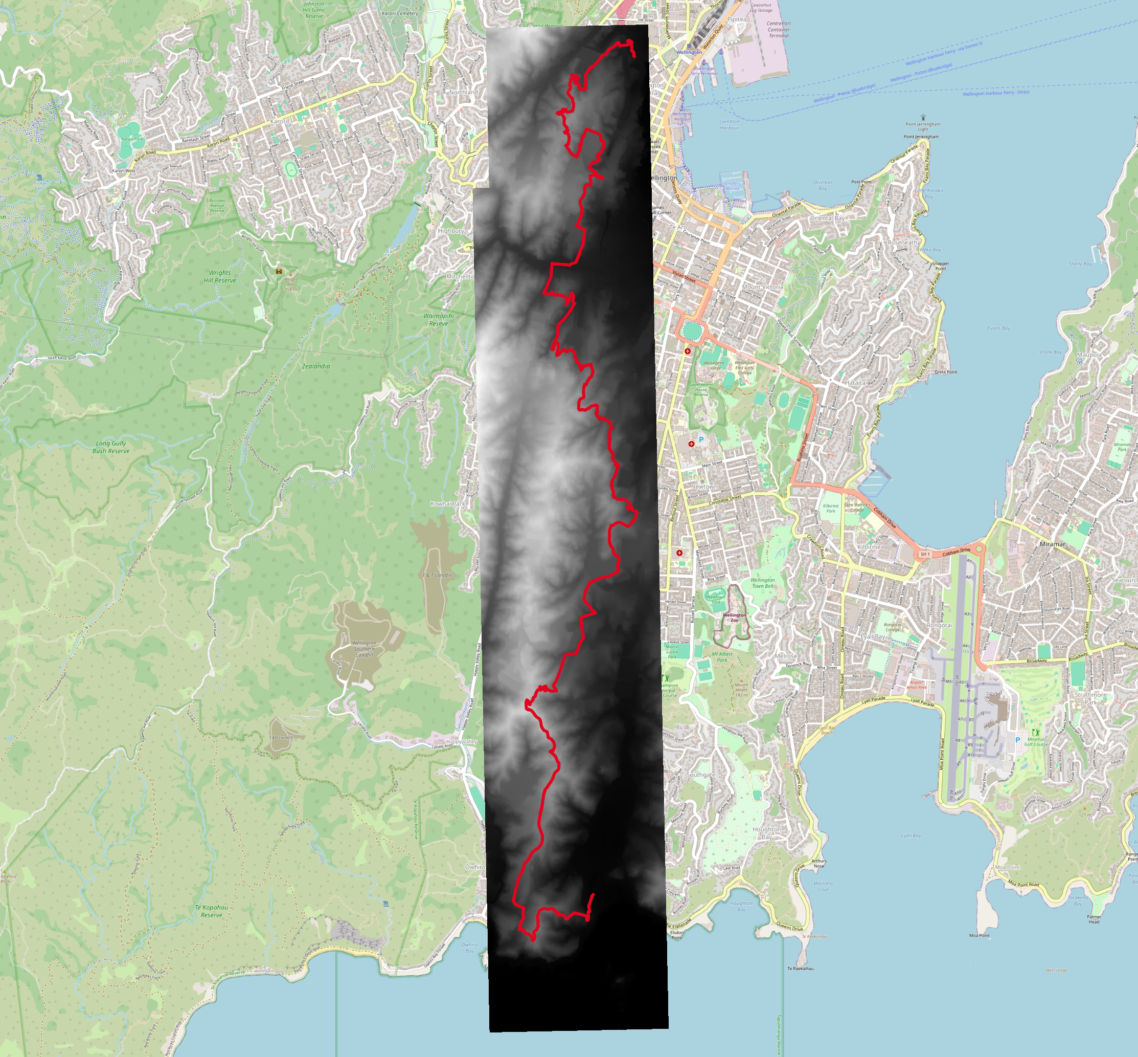
library(patchwork)

When a route is not a linestring

Turns out this was a little more complicated than I expected. If I’d been smart I’d have tracked my tramp on my phone and thus have had a single sequence of points that could be made into a single linestring which is what’s needed to make an elevation profile. I didn’t think to do that and was instead faced with the multilinestring available via OpenStreetMap (downloaded using the excellent QuickOSM plugin for QGIS).

That’s what’s shown in the thrown together map above. And that’s fine if all you want to do is put a line on the screen. If you want to interpolate points along a line then you need a single linestring, and it’s not always the case that multilinestrings can be trivially converted into linestrings.

It turns out that this particular multilinestring is well behaved and can be combined into a single linestring using st_line_merge. I’ve shown an example at the end of this post where this is not the case.

city_to_sea <- st_read("city-to-sea-all.gpkg") |>
  st_transform(2193) |>
  st_line_merge()

Making an elevation profile

Now that we have a single linestring, we also need elevation data. This is extracted from Wellington LiDAR imagery available here.

dem <- rast("c2s.tif")
names(dem) <- "Elevation"

We can make a profile by sampling at equally spaced intervals along the linestring usingst_line_interpolate and terra::extract. The walkway is about 14.5 km, so 3000 steps is roughly every 3m. That seems about right when the elevation data is at 1m resolution.

steps <- 0:3000 / 3000

points <- city_to_sea$geom |>
  st_line_interpolate(steps, normalized = TRUE)

profile <- terra::extract(dem, points |> as("SpatVector")) |>
  mutate(Distance = (city_to_sea |> st_length()) * steps) |>
  mutate(Distance = drop_units(Distance))

1

normalized = TRUE means that 0 is the start of the line and 1 is the end of it.

2

It’s easier to work with distances presented as plain numbers not units.

And now we can make a plot of elevation by distance along the walk. It’s instructive here to show the elevation and distance at the same scale, and also with the elevation exaggerated eight-fold. The at-scale version is that barely visible horizontal sliver. Clearly, in some sense, this walk is not as hilly as it feels!

g_profile_1 <- ggplot() +
  geom_area(data = profile, aes(x = Distance, y = Elevation), fill = "grey") +
  coord_fixed() +
  theme_minimal()

g_profile <- ggplot() +
  geom_area(data = profile, aes(x = Distance, y = Elevation), fill = "grey") +
  coord_fixed(ratio = 8) +
  theme_minimal()

(g_profile_1 / g_profile & labs(x = NULL, y = NULL)) + 
  labs(x = "Distance", y = "Elevation")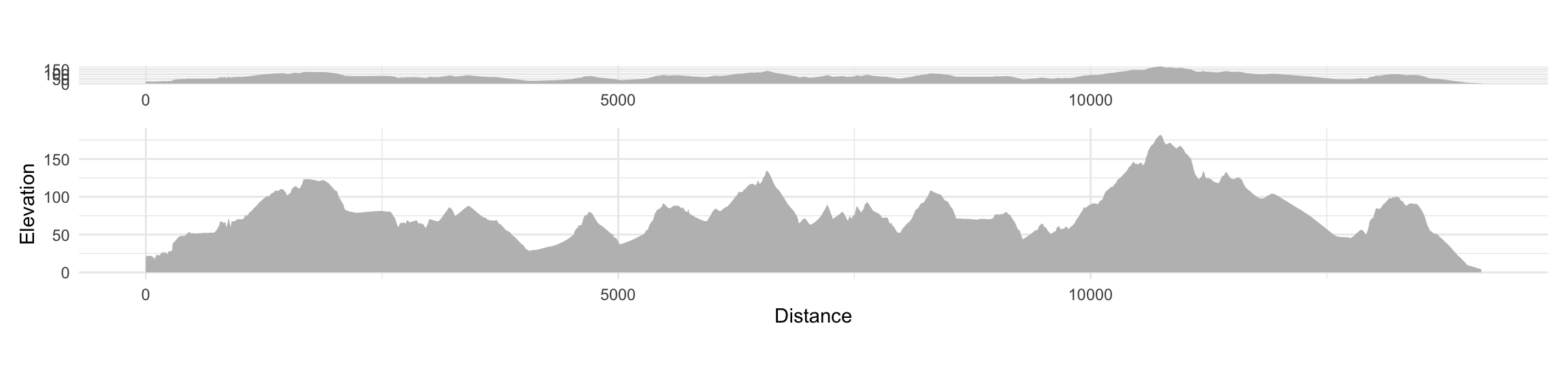

Figure 2: Elevation profile of the City to Sea Walkway shown at scale, and with elevation exaggerated eight-fold.

Adding some names to the walkway segments

Named City to Sea segments are also available from OpenStreetMap. We can use these to add some contextual information to our elevation profile.

named_segments <- st_read("city-to-sea-segments.gpkg") |>
  st_transform(2193) |>
  select(name) |>
  filter(!is.na(name) & name != "City to Sea Walkway") |>
  group_by(name) |>
  filter(row_number() == 1)

1

Any name attribute that is ‘City to Sea Walkway’ is not very useful in this context, so we drop those.

2

The last two steps remove duplicate names retaining only the first instance of any name that appears more than once.

Next we convert the line segments to points half way along the segment length and add to each point its distance along the city_to_sea linestring.

named_points <- named_segments |>
  mutate(geom = st_line_interpolate(geom, 0.5, normalized = TRUE),
         Distance = st_line_project(city_to_sea$geom, geom))

And now, as before we find the elevation of each of these points. I also make a simple dataframe version of the data so we can plot the data based on the distance and elevation rather than the planimetric map coordinates.

named_points <- bind_cols(
  named_points, 
  named_points |>
    as("SpatVector") |>
    terra::extract(x = dem, method = "bilinear", ID = FALSE))

name_xys <- named_points |> 
  st_coordinates() |>
  data.frame() |> 
  rename(x = X, y = Y) |>
  bind_cols(named_points |> st_drop_geometry())

And now we can make a labelled version of the elevation profile.

g_profile_labelled <- g_profile + 
  geom_text(
    data = name_xys, 
    aes(x = Distance, y = Elevation, label = name),
    angle = 90, size = 2.5, hjust = 0, vjust = 0.5, nudge_y = 5, 
    check_overlap = TRUE) +
  scale_y_continuous(breaks = seq(0, 150, 50)) +
  coord_fixed(ratio = 8, ylim = c(0, 350)) +
  theme(axis.title.y = element_text(hjust = 0.15))
g_profile_labelled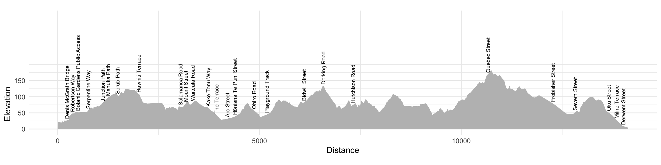

Figure 3: The profile with labelled locations based on names of segments.

Making an actual map

I could argue that this elevation profile is a map, but my heart wouldn’t really be in it. Instead, it’s fun to make a parallel map of the path, and roughly line the two up next to one another. Because the elevation profile is ‘landscape’ mode, I want the map to also be oriented with its long axis horizontal. Given the very strong north-south orientation of the walkway, it’s convenient to do this by a coordinate swap, so here is a function for that.

switch_xy <- function(df) {
  df |>
    mutate(z = -y, y = x, x = z) |>
    select(-z)
}

1

To swap the x and y coordinates we need a temporary third attribute, which I’ve imaginatively called z.

2

And since it’s temporary, we throw it away.

I explored doing this with an actual map projection or by faking a projection using matrix multiplication¹, but in the end decided it was easier just to convert my data to plain dataframes with x and y attributes and alter those as needed.

The 1m resolution DEM is more detail than we really need, so I aggregate it and make a hillshade, which, because I’m using ggplot for mapping I also convert into a simple dataframe, and switch the coordinates.

dem_x5 <- dem |> aggregate(5)
slope <- dem_x5 |> terrain(unit = "radians")
aspect <- dem_x5 |> terrain(v = "aspect", unit = "radians")
hillshade <- shade(slope, aspect, direction = 225) 
hillshade_yx <- hillshade |>
  as.data.frame(xy = TRUE) |>
  switch_xy()

We also need the route and named points as dataframes, with coordinates swapped.

name_yxs <- name_xys |>
  switch_xy()

city_to_sea_yx <- city_to_sea |> 
  st_coordinates() |> 
  data.frame() |>
  select(X, Y) |> 
  rename(x = X, y = Y) |>
  switch_xy()

xmin <- min(hillshade_yx$x)
ymax <- max(hillshade_yx$y)

And finally we can make the map with the elevation profile underneath. There’s a bit of fiddle here with positioning of annotations, and to make a north-arrow, something I am usually reluctant to provide, but which in this case, given the wilfull reorientation by 90° seems warranted.

g_map <- ggplot() +
  geom_raster(
    data = hillshade_yx,
    aes(x = x, y = y, fill = hillshade), alpha = 0.5) +
  scale_fill_continuous_c4a_seq(palette = "brewer.greens") +
  guides(fill = "none") +
  geom_path(data = city_to_sea_yx, aes(x = x, y = y),
            linetype = "dashed") +
  geom_text(
    data = name_yxs, aes(x = x, y = y, label = name),
    angle = 90, size = 2.5, hjust = c(rep(0:1, 15), 0), vjust = 0.5, 
    nudge_y = c(rep(c(25, -25), 15), 25), check_overlap = TRUE) +
  annotate("segment",
    x = xmin + 250, y = ymax + 100,
    xend = xmin + 150, yend = ymax + 100,
    arrow = arrow(type = "closed",
                  length = unit(0.1, "npc"), angle = 20)) +
  annotate("text",
    x = xmin + 80, y = ymax + 100, label = "N", size = 5) +
  coord_equal(ylim = range(hillshade_yx$y) + c(-200, 250)) +
  ggtitle("Wellington's City to Sea Walkway") +
  theme_void()

1

A home-made north arrow.

2

And the necessary ‘N’.

Finally put the two together with patchwork.

(g_map / g_profile_labelled) + 
  plot_layout(heights = c(5, 4))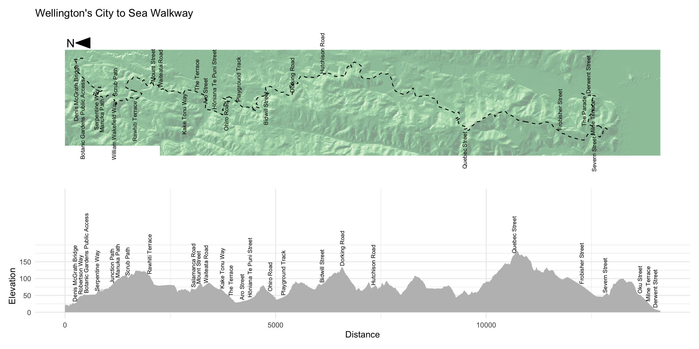

Figure 4: Roughly aligned map and elevation profile of the route.

They’re not entirely aligned, but then again, a precise alignment is impossible since the path is twisty and therefore non-uniform in terms of the relationship between progress from city (in the north) to sea (in the south) versus elapsed distance along the path.

A more annoying issue is that because the labels are placed differently in each representation the check_overlap filter in each plot has chosen a different set of labels to keep. A better approach might would likely be to hand pick the labels to include, and ensure that all of the selected labels appear in both plots. That wouldn’t be too hard to arrange, but I’m happy enough with this version and will leave it as is.

Addendum: making a linestring from messier data

Above I made the unified linestring representation of the City to Sea Walkway from an input file containing a single multilinestring. The version of the data with named segments on the walk turns out to be less cooperative than that.

segments_2 <- st_read("city-to-sea-segments.gpkg") |>
  st_transform(2193) |>
  st_cast("LINESTRING")

This dataset doesn’t play ball when I try to combine it into a single linestring using st_line_merge:

segments_2 |> 
  st_union() |>
  st_line_merge() |>
  st_cast("LINESTRING")

Geometry set for 5 features 
Geometry type: LINESTRING
Dimension:     XY
Bounding box:  xmin: 1747444 ymin: 5421285 xmax: 1748604 ymax: 5428814
Projected CRS: NZGD2000 / New Zealand Transverse Mercator 2000

We don’t get a single linestring; instead we get five. The reason is that this dataset has a couple of small branch sections. We can detect these by counting how many other segments each segment touches.

connections <- segments_2 |>
  st_touches(remove_self = TRUE)

n_connections <- connections |> 
  lengths()

table(n_connections)

n_connections
  1   2   3 
  3 137   3 

If the collection of linestrings formed a single linear chain, we’d expect there to be no linestrings that touch three others, and only two (one at the start, and one at the end) that touch only one other. We can map this (although you’ll have to squint to see the ‘spurs’ or ‘on-ramp’ segments, that are causing the problem—click on the map for a closer look).

segments <- segments_2 |>
  st_coordinates() |>
  data.frame() |> 
  left_join(data.frame(L1 = 1:143, n = as.factor(n_connections)))

ggplot(segments) +
  geom_path(aes(x = -Y, y = X, group = L1, colour = n)) +
  scale_colour_manual(values = c("red", "grey", "dodgerblue")) +
  theme_void()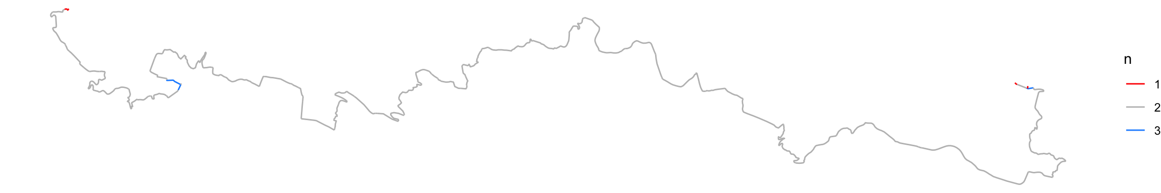

Figure 5: A map showing the ‘rogue’ segments

To piece together a maximal single linear route in this case we can proceed as follows. First, determine which segments in the route touch, and use those relations to build a graph.

G <- segments_2 |> 
  st_touches(sparse = FALSE) |>
  graph_from_adjacency_matrix(mode = "undirected")

Now, find the longest shortest path in the graph (in graph terms, its diameter). This connects the most remote ends of the graph, which we assume will give us appropriate start and end points for the whole of the City to Sea Walkway.

D <- distances(G)
start_finish <- which(D == max(D), arr.ind = TRUE)[1, ]
start_finish

row col 
140  21 

Now, we get the shortest path, i.e. the list of segments between those two end segments…

route <- shortest_paths(
    G, start_finish[1], start_finish[2])$vpath |>
  unlist()

… and then use that list of segments to slice the named_segments dataset and assemble the route using st_line_merge.

city_to_sea_2 <- segments_2 |>
  slice(route) |>
  st_union() |>
  st_line_merge()

And here’s a very quick and dirty map to check we successfully extracted the ‘trunk’ of the walkway.

ggplot() +
  geom_path(data = city_to_sea_2 |> st_coordinates() |> data.frame(),
            aes(y = X, x = -Y)) +
  coord_equal() +
  theme_void()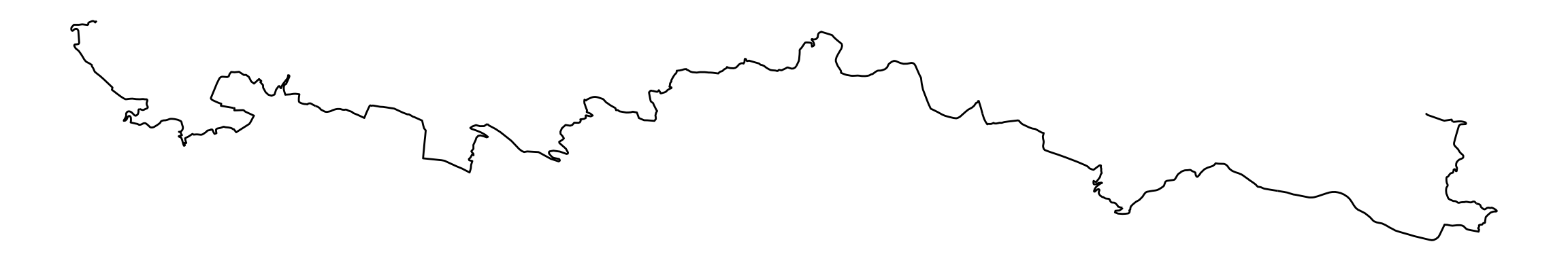

Figure 6: A quick and dirty map of the main trunk route of the walkway.

Footnotes

1. I have previous on that score as regular readers if I have any will know…