Into the void

A couple of weekends ago I walked the Paparoa Track, one of New Zealand’s Great Walks. It was indeed great, although we got thoroughly soaked on days two and four of our afternoon, two days, and a morning sojourn. The West Coast Region is famously wet, being not at all in the rain shadow of the Southern Alps (quite the reverse) with around 3m of rain a year. There is also no obvious discernible difference between the seasons in terms of monthly precipitation,¹ so we should have expected as much.

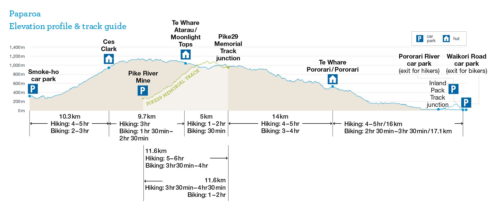
The Department of Conservation provides good guidance on the elevation profile of the track, which is dual use hiking and mountain-biking, and so has been graded so that it’s rarely steeper than 6%. Given the ruggedness of the terrain, the track is astonishingly level, and much easier going metre for metre than (say) Wellington’s City to Sea Walkway or pretty much anywhere in the Tararuas. There was great information in one of the huts about the construction of the track, and it really is an engineering marvel, that nevertheless somehow seems natural. For all that, I am happier to have been walking it than biking it, given some of the narrow sections and precipitous drops.

Figure 1: Department of Conservation informational posters about the track construction photographed in one of the huts.

Given the virtual whiteout on two of our days we didn’t get to appreciate the promised expansive views or sunsets, so I thought it would be interesting to get a feel for what we might have been able to see on clearer days.

library(terra)
library(sf)
library(tmap)
library(dplyr)
library(stringr)
library(igraph)

Data

Although Lidar data are available for West Coast, for an area of this extent the associated files are enormous. Instead I’ve used the 15m resolution School of Surveying DEM available here, cropped to an area fairly closely around the track. On those promised clear days the Southern Alps are apparently visible, but that would demand still more data, so perhaps another time.

Track and huts data were obtained from OpenStreetMap using the QuickOSM plugin. Unfortunately, it took quite a lot of editing in QGIS to clean up the track data and focus only on the Paparoa Track walking route.

dem <- rast("nzsosdem.tif")
sea <- is.na(dem)

slope <- dem |> terrain(unit = "radians")
aspect <- dem |> terrain(v = "aspect", unit = "radians")
shade <- shade(slope, aspect, direction = 135)

dem <- dem |> mask(sea, maskvalues = TRUE)
shade <- shade |> mask(sea, maskvalues = TRUE)

track <- st_read("paparoa-track.gpkg")
huts <- st_read("huts.gpkg")

Data loaded, we can assemble a simple map of the track.

m_base <- 
  tm_shape(sea) +
  tm_raster(
    col.scale = tm_scale_categorical(values = c("white", "lightblue2")),
    col.legend = tm_legend_hide()) +
  tm_shape(dem) + 
  tm_raster(
    col.scale = tm_scale_continuous(
      values = "hcl.terrain2", limits = c(0, 3000)),
    col_alpha = 0.6, 
    col.legend = tm_legend_hide())

m_shade <- 
  tm_shape(shade) +
  tm_raster(
    col.scale = tm_scale_continuous(values = "brewer.greys"),
    col_alpha = 0.2, 
    col.legend = tm_legend_hide())

m_tracks_and_huts <-
  tm_shape(track) +
  tm_lines(col = "red3", lty = "dashed", lwd = 1.5) +
  tm_shape(huts) +
  tm_dots(col = "white", fill = "red3", shape = 22, size = 1)

m_labels <-
  tm_shape(huts) +
  tm_text(
    text = "name", ymod = 0.75, size = 0.9,
    options = opt_tm_text(just = c("center", "bottom")))

m_scalebar <- 
  tm_scalebar(
    text.size = 0.75,
    position = tm_pos_out(cell.h = "center", cell.v = "bottom",
                                    pos.h = "center", pos.v = "top"))

m_base + m_shade + m_tracks_and_huts + m_labels + m_scalebar

Figure 2: General location map of the Paparoa Track

You get some sense of the tortuously twisty nature of the track by noting that the route is 56km, yet the crow’s flight end-to-end distance at about 26km is less than half of that.

We walked from south to north, stopping for a night at each of the huts shown in the map. The distances covered each day were roughly 10km, 10km, 19km, and 16km, respectively. The toughest in terms of exertion was day 1 which was more or less all uphill. Day 2, when the weather set in was not a lot of fun, although it gave us good reason to be thankful for the well constructed track’s astonishing drainage.². Day 3 dawned promising more of the same, but cleared later in the day so we did get some great views from the Pororari Hut. Day 3 also featured some amazing and quite unheralded waterfalls en route—the kind of waterfalls that in other contexts would have a 500 car park at the bottom and a constant stream of visitors. Day 4 was wet again, but downhill all the way, and while sightlines were limited, the rainforest and Pororari River gorge were spectacular.

Which hut has the ‘best’ views?

On our tramp, the Pororari Hut had the undisputed best views because that afternoon and evening was by some margin the best weather of the trip. We were even able to see back to the Moonlight Tops Hut, albeit only briefly, before the mist rolled across that hut again).

But how would the views from the huts compare on theoretical³ clear days?

This isn’t a difficult question to address, at least in terms of extent of the views available from any given spot.

viewsheds <- list()
for (i in 1:nrow(huts)) {
  viewsheds[[huts$name[i]]] <- 
    dem |> viewshed(huts$geom[i] |> st_coordinates(), observer = 5)
}
viewsheds <- rast(viewsheds)

And we can map the viewsheds for comparison, shrouding the areas hidden from view at each hut in an appropriately dense grey fog.

m_viewsheds <- 
  tm_shape(viewsheds) +
  tm_raster(
    col.scale = tm_scale_categorical(values = c("#eeeeeea0", "#ffffff00")),
    col.legend = tm_legend_hide())

m_base + m_shade + m_viewsheds + m_tracks_and_huts + m_labels

Figure 3: Maps of the viewsheds from the three huts

According to this analysis the Pororari Hut has the most extensive views. I’m not entirely convinced by this, and suspect that on really clear days the views to the south and east from the other two huts might outshine those from Pororari. Saying that, they weren’t bad.

Figure 4: A view from Pororari Hut according to a bad smartphone camera.

View points along the track

It’s not all about the huts, of course. I think we all feel we missed out on the section between Ces Clark and Moonlight Tops, which is essentially a ridge line the whole way, but for us a stretch where visibility was rarely much beyond (say) 50 metres.

We can explore how the viewshed from points along the track varies along its length. To do so, as in a previous post, the track linestrings have to be combined into a single linestring. Click into the code block below to see how that can be done.

linestring_as_matrix <- function(L) {
  (L |> st_coordinates())[, 1:2]
}

join_segments <- function(s1, s2) {
  junction <- st_intersection(s1, s2)
  along_1 <- st_line_project(s1, junction, normalized = TRUE)
  along_2 <- st_line_project(s2, junction, normalized = TRUE)
  m1 <- linestring_as_matrix(s1)
  m2 <- linestring_as_matrix(s2)
  if (along_1 == 0) {
    m1 <- apply(m1, 2, rev)
  }
  if (along_2 == 0) {
    m2 <- m2[-1, ]
  } else {
    m2 <- apply(m2, 2, rev)[-1, ]
  }
  st_linestring(rbind(m1, m2)) |> 
    st_sfc() |>
    st_set_crs(st_crs(s1))
}

segments <- track |>
  st_cast("LINESTRING")

connections <- segments |>
  st_touches()

start_finish <- which((connections |> lengths()) == 1)

sequence <- (segments |> 
               st_touches(sparse = FALSE) |>
               graph_from_adjacency_matrix(mode = "undirected") |>
               shortest_paths(from = start_finish[1], to = start_finish[2]))$vpath |>
  unlist()

single_track <- segments$geom[sequence[1]]
for (i in sequence[-1]) {
  single_track <- join_segments(single_track, segments$geom[i])
}

That done we can take snapshots at points equally-spaced along the track.

viewpoints <- ((0:200) / 200) |> 
  st_line_interpolate(line = single_track, normalized = TRUE) |>
  as.data.frame() |>
  st_as_sf()
sheds <- list()
view_scope <- c()
for (i in 1:nrow(viewpoints)) {
  sheds[[i]] <- viewshed(dem, viewpoints$geometry[i] |> st_coordinates()) * 1
  view_scope <- c(
    view_scope,
    sheds[[i]] |> values() |> sum(na.rm = TRUE)
  )
}
sheds <- rast(sheds)
names(sheds) <- str_c("v", 0:200)

Of these viewpoints, which offers the most expansive views? We can pick that spot out easily and map the associated viewshed.

i <- which.max(view_scope)
m_base + 
  m_shade + 
  tm_shape(sheds[[i]]) +
  tm_raster(
    col.scale = tm_scale_categorical(
      values = c("#eeeeeea0", "#ffffff00")),
    col.legend = tm_legend_hide()) + 
  m_tracks_and_huts +
  tm_shape(viewpoints |> slice(i)) +
  tm_dots(size = 1, shape = 19)

Figure 5: The maximum viewshed along the track.

The stack of viewsheds sheds can also tell us which location across the study area is most visible, i.e., most often visible from some the points we’ve ranged along the track.

prominence <- sheds |> sum()

tm_shape(prominence) +
  tm_raster(
    col = "dodgerblue",
    col_alpha = "sum",
    col_alpha.scale = tm_scale_continuous(),
    col_alpha.legend = tm_legend_hide()) + 
  m_shade + 
  m_tracks_and_huts

Figure 6: General location map of the Paparoa Track

The most prominent locations (in pale blue), are ridge lines parallel to and close to the track for parts of its length.

And finally…

I used the code below to make a video of the evolving extent of the viewshed along the track. If you happen to run this be aware that it is not quick, taking 20+ minutes.⁴

maps <- list()
for (i in 1:201) {
  maps[[i]] <- m_base + 
    m_shade +
    tm_shape(sheds[[i]]) +
    tm_raster(col.scale = tm_scale_categorical(values = c("#eeeeeea0", "#ffffff00")),
              col.legend = tm_legend_hide()) + 
    m_tracks_and_huts +
    tm_shape(viewpoints |> slice(i)) +
    tm_dots(size = 1, shape = 19)
}
tmap_animation(maps, "paparoa-viewsheds.mp4", width = 1000, height = 1600, delay = 20)

Figure 7: Video of the evolving viewshed along the track at approximately 250 metre intervals.

All told, I’d say we saw about 1/10th of that, although we still had a great time!⁵

Footnotes

1. In fact, December seems to be the wettest month on average… keep in mind that’s the summer here.

2. The track itself was practically a river on Day 2, but with regular channels to drain that water off to the sides

3. Very theoretical…

4. Admittedly on a Macbook Air running on battery.

5. ⭐⭐⭐⭐⭐ would recommend.