Maps of all the possible air routes where the origin and destination airport IATA codes would differ by only one letter, and of the ones that actually do. Also, grobs.
geospatial
r
tutorial
networks
ggplot
life
Author
David O’Sullivan
Published
June 27, 2025
Last year some time I found myself on a flight from Dubai (DXB) to Dublin (DUB) and of course my pattern detecting brain noted the off-by-one-letter difference in the International Air Transport Association (IATA) codes of the two airports. It got in my head at the time and between watching bad movies and dozing and wondering if the flight would ever end (it was the third leg of a WLG - AKL - DXB - DUB endurance test) I found myself idly wondering, just how many off-by-one-letter flights there are. Are they rare or commonplace? Where are they? How many could there possibly be?
So, for all those similarly afflicted by such questions, here’s a post with more than you ever wanted to know about this deeply trivial matter. As always, there are coding tricks to be learned along the way. The code I think is less interesting can also be viewed by clicking on the ▸ Code links.
For densifying points along meridians to make a ‘globe’ polygon.
We need some base world data, and I’ve also made a ‘globe’ so we can colour in the background sensibly in a non-rectangular projection. I’ve chosen 30°E for the central meridian of my world maps because1 that allows all the off-by-one routes that exist to be shown without breaks.
Using a central meridian 30°E gives a better centred final map.
2
Break things based on a central meridian 30°E
3
For rounded ‘edges’ to the globe when projected.
Aviation data
Via ourairports.com2 we can get pretty comprehensive data on airports, large and small. So much data in fact (some 83,210 airports) that I’ve limited the focus for this post to a mere 482 ‘large’ airports that also have an IATA code.
Finding the best way to get all the two airport combinations proved trickier than I expected, at least it did for as long as I persisted with trying to do it ‘tidily’. I also took a detour via igraph which allows for a nice graph-based approach, round-tripping airport-pairs via a simple undirected graph. That’s appropriate in some respects, but really overkill for this problem. Knowing when to give up is half the battle, and switching to using base R’s combn is simple, give or take a bit of matrix conversion to get the results into a dataframe.
After that it’s a simple matter to filter for routes with a Hamming distance between codes as calculated by stringdist of exactly one, and then join coordinate data for the two airports.
While flights might very well not follow great circle routes in all cases, they are the most appropriate general way to represent them on a world map, which is where geosphere comes in.
The tricky part here was to break the great circle linestrings into multistrings at my chosen antimeridian, 150°W. While sf::st_break_antimeridian does this correctly, for reasons that I think are associated with the various format conversions from old style spatial data generated by geosphere to sf I wound up with duplicate copies of every flight that crosses the anti-meridian, in addition to a multilinestring broken at the meridian. Fixing this requires a couple of additional steps.
Add a "AKL-WLG" style route attribute to help in identifying duplicate routes.
2
Group on the route attribute and summarise to create multilinestrings. This is the retrospective fix for extra linestrings that showed up in the previous step.
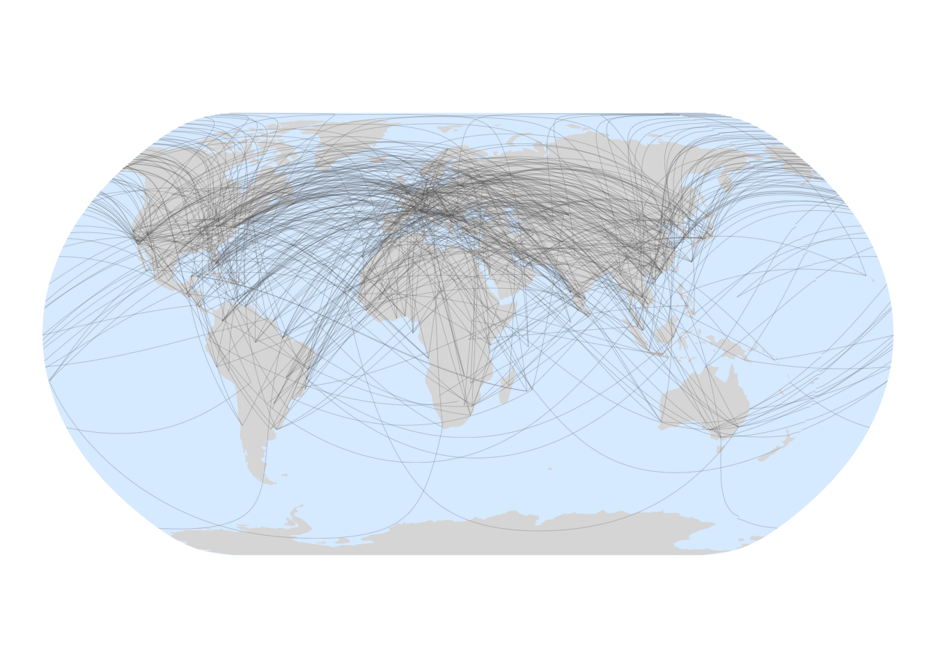
Figure 1: All possible routes between major airports differing by one letter in their IATA codes.
Just to emphasise: this is not a map of actually existing off-by-one routes, it’s a map of all the 782 possible such routes between our 482 large airports. That’s from a possible 116,402 routes, or about 0.67%. This is more than half as many again as we’d expect if the codes were random. There are up to 26-cubed or 17,576 codes. Any given code can connect to as many as 17,575 other codes, and of these only 75 can be off-by-one (there are 25 possible different letters in each of the three available positions). That’s 75 / 17,575, which is only 0.43%
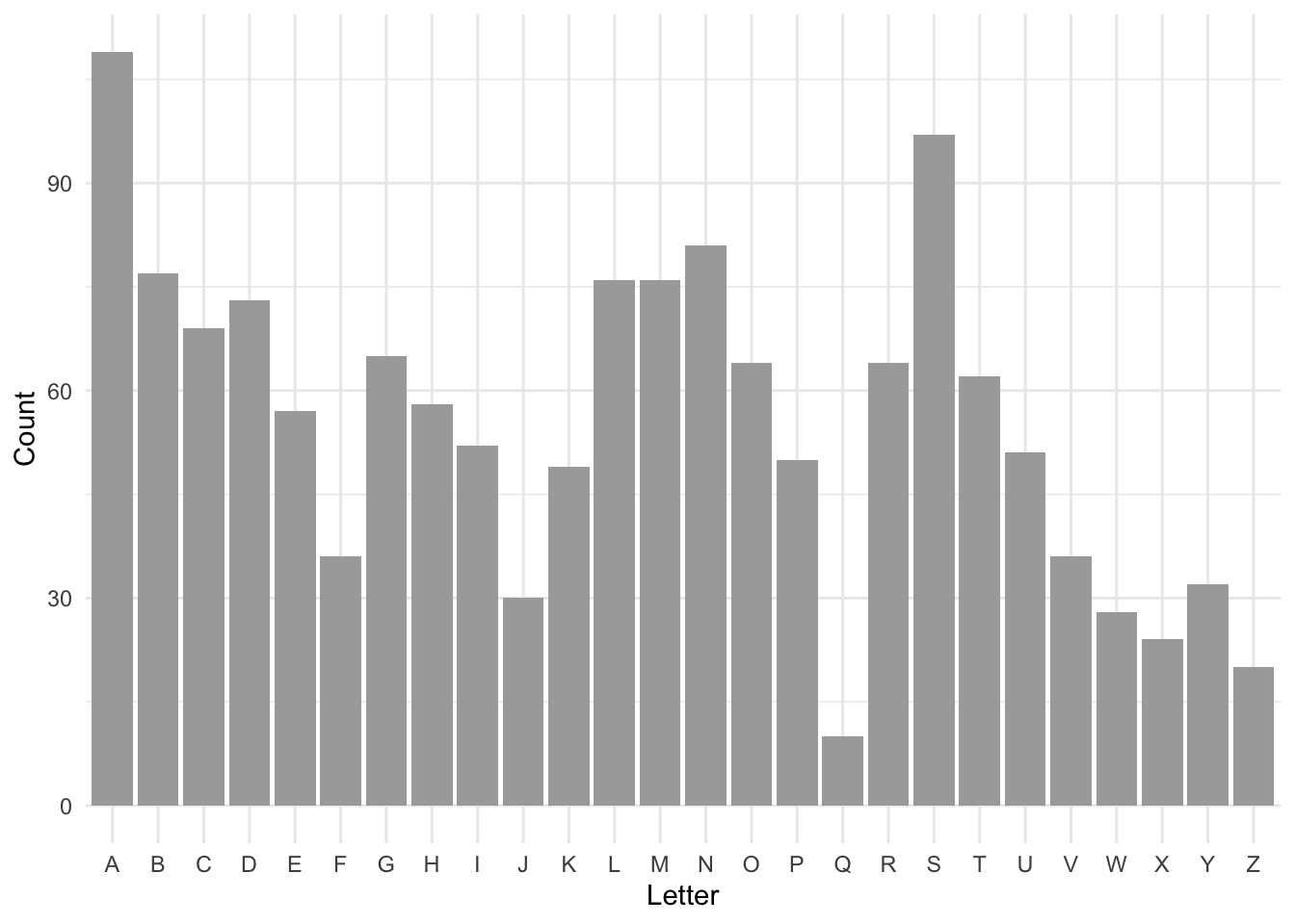
Of course the codes aren’t random, they generally bear some relation to the names of actual places3 and we’d therefore expect the distribution of letters in the codes to be uneven. We can confirm this very easily:
Code
letter_freqs =data.frame(Letter = LETTERS,Count = airports |>pull(iata_code) |>str_c(collapse ="") |>str_count(LETTERS))ggplot(letter_freqs) +geom_col(aes(x = Letter, y = Count), fill ="darkgrey") +theme_minimal()
1
LETTERS and letters are vectors of the alphabet in upper and lower case. A handy thing to know.
Figure 2: Counts of letters in the IATA codes of 482 airports
I checked for the 9000 or so airports that have codes and the pattern is not so different, with A and S still the most favoured letters.
Sadly, it’s difficult to source open data on regularly scheduled flights, because it’s commercially valuable information. The best I could do was from openflights.org, but as they say “The third-party that OpenFlights uses for route data ceased providing updates in June 2014”.5 Anyway, we can filter out routes from our off-by-one dataset that don’t appear in this list.
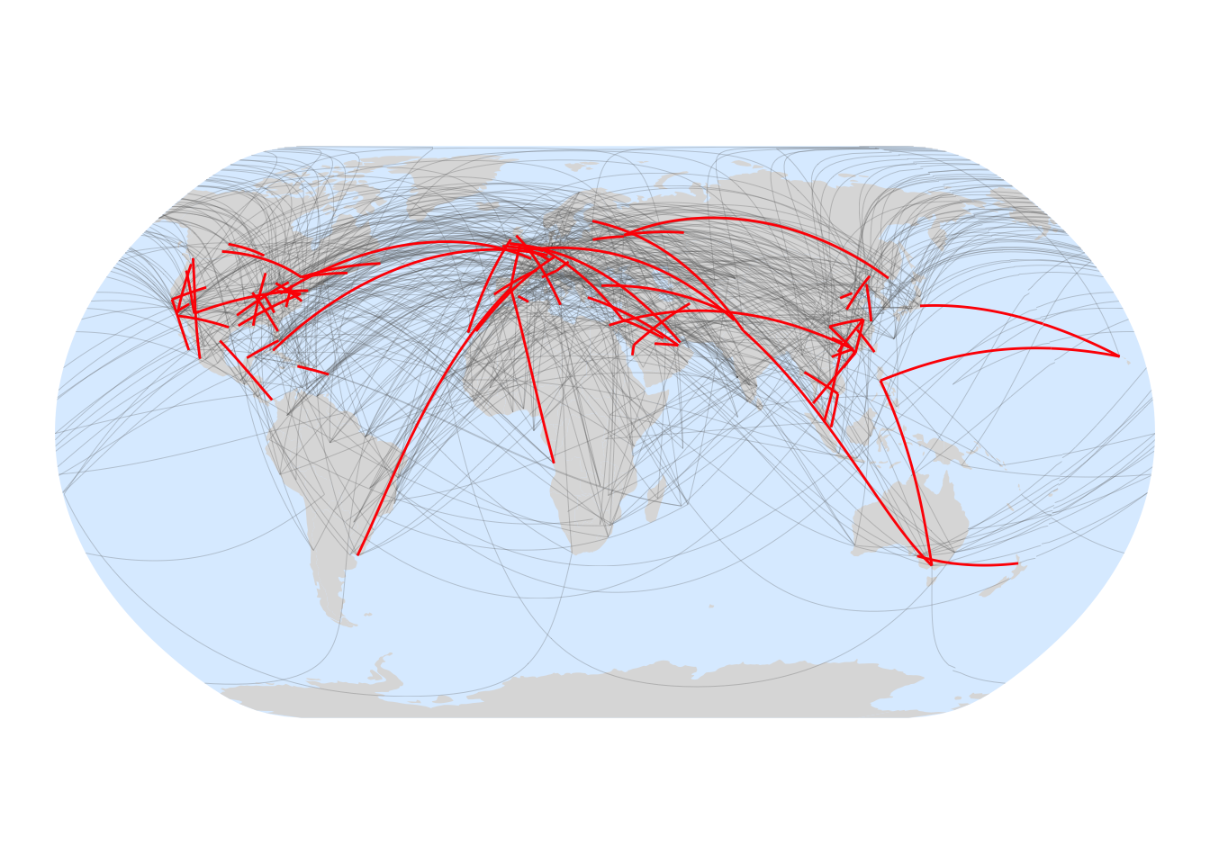
Figure 3: Actually existing routes off-by-one in their IATA codes highlighted in red.
The longest of these routes is Melbourne (MEL) to Delhi (DEL) from where you could get an onward connection to Helsinki (HEL). Surprisingly New Zealand’s only entrant in this list is the relatively local Auckland (AKL) to Adelaide (ADL). Amusingly, the shortest off-by-one route at 324km is between King Abdulaziz International Airport (JED) and Prince Mohammad Bin Abdulaziz Airport (MED) both in Saudi Arabia, and keeping airport naming rights in the family.
More local maps
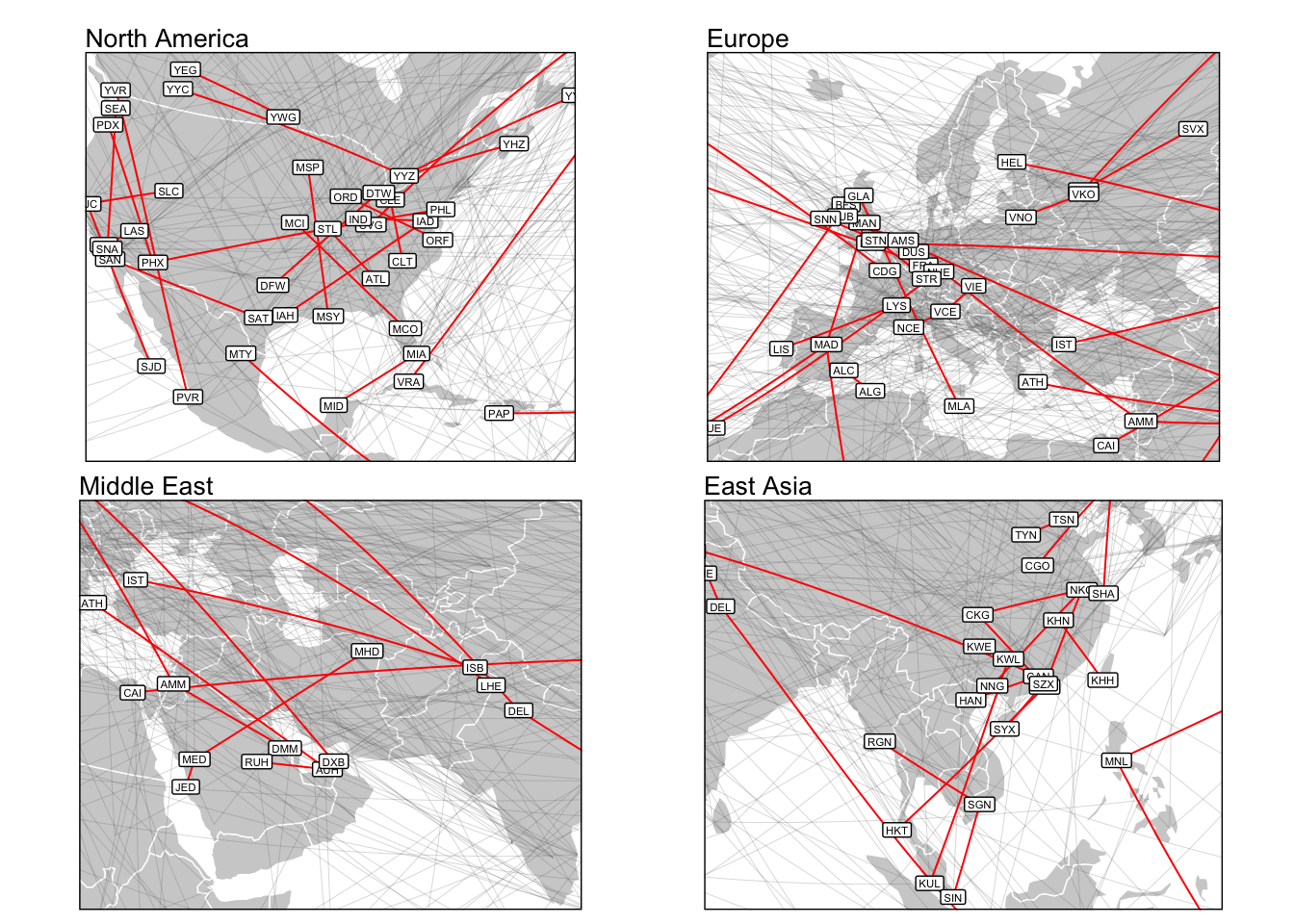
In lieu of a zoomable web map6 below are four more localised views.
No lat_0 is required for this projection, but might be if I change it some time.
2
It’s necessary to ‘cast the net wide’ to make sure all countries within a window in lat-lon are on the map in the projected space, which is quite different than the lat-lon bounding box.
3
Returning plots as plots caused me some memory issues, which seem to be resolved by returning them as ‘grobs’. There’s a first time for everything in my R journey.
Figure 4: Regionally focused maps with IATA codes shown.
Finally: are the off-by-one routes clustered?
It’s not easy to know exactly how to approach this question. But we might expect, due to geographical patterns in naming and language, that there would be some clustering of the actual off-by-one routes. A rough and ready approach to testing this idea is applied in the code cell below, based on the lengths in km of the various subsets of flights. The idea is that shorter length routes might be more common among off-by-one routes than in scheduled flights in general.
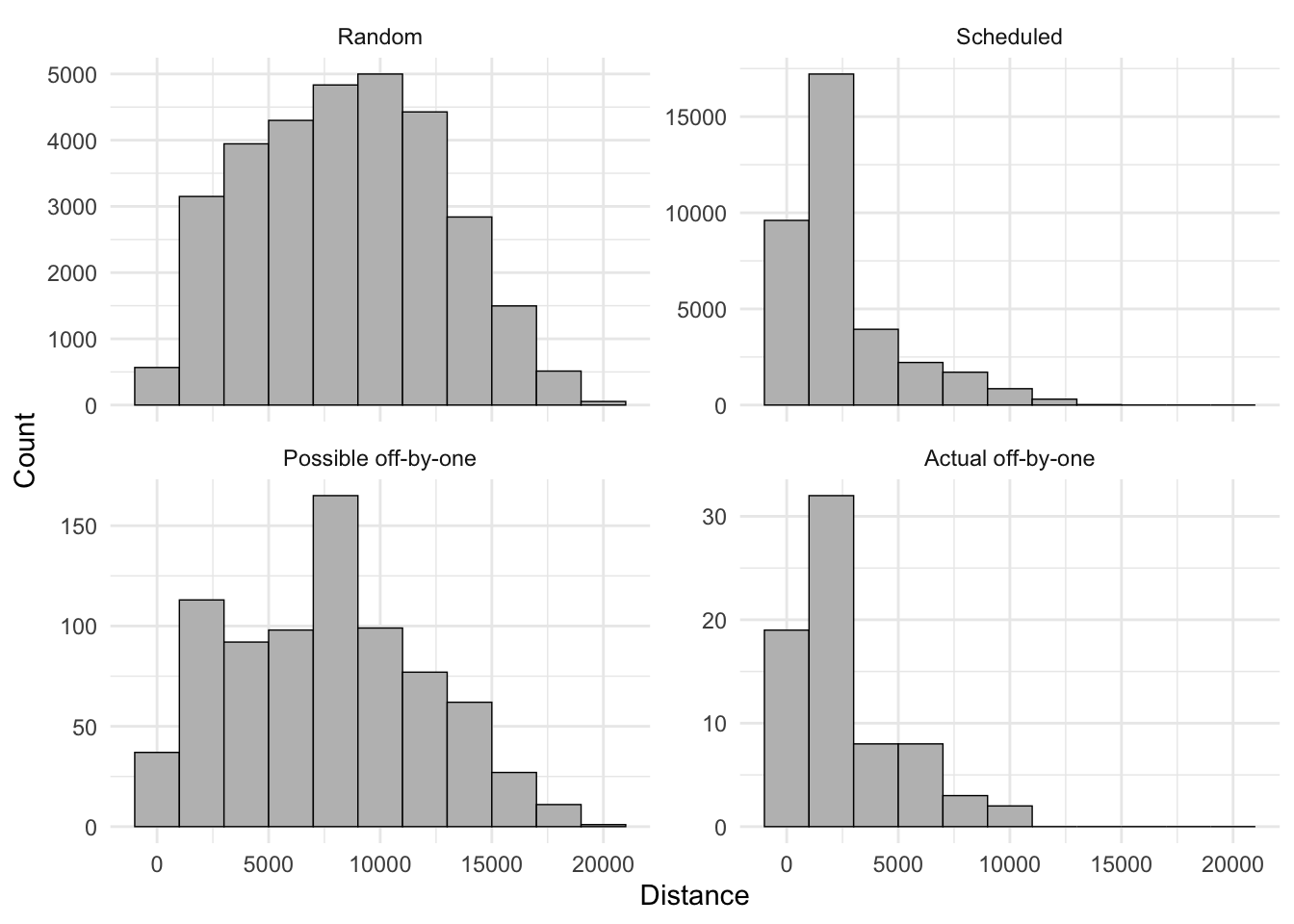
Figure 5: A comparison of the flight length distributions of each category of flight.
Looking at these distributions there’s no reason to think there’s any geographical patterning, in spite of Canada’s attempt to tip the scales with its weird Y– codes.7
Completely random flights with origins and destinations randomly located on land (excluding Antarctica) and our all possible off-by-one flights are similarly distributed, although the latter has a spike in shorter (sub-5000 km) flights and another around 8000 km. These are most likely due to unevenness in population densities and hence airports relative to my naïve null model. For example, larger numbers of short flights than the null model shows are likely within-region flights, while the spike around 8000 km is probably trans-oceanic flights between densely populated coastal areas. A more sophisticated ‘null’ model would position random airports based on population densities, and perhaps demonstrate this characteristic, but that seems a bit like overkill in this context! Both these distributions include entirely unrealistic and irrelevant flights longer than 15,000 km which simply don’t exist.8
Meanwhile, the lengths of actually existing off-by-one flights look very much like a random sample from the lengths of all scheduled flights. Based on this evidence it would be hard to make a claim that there’s any geographical pattern to where you are most likely to find yourself on one of these flights. A code after all is just a code, especially when, like IATA codes it has developed in an ad hoc manner with a need for consistency locking in many early decisions, unlike, for example, the numbers assigned to highways in the United States and roads in the United Kingdom based on explicitly geographical schemes.
So next time, if ever, you find yourself on one of these rare-ish 1-in-150 flights, do your best to appreciate it. But there’s really no need to add this to your bucket list. Saying which, MEL-DEL-HEL seems like it could be… fun?
I regret to say I’ve been on a couple of these, a side-effect of being from Ireland and living in New Zealand. I can’t recommend such super-long flights in economy unless it’s in an A380. But can I just say? Those things are awesome.↩︎
Oh well, never mind. This is a fun little project but not one worth spending any money on.↩︎
Which comes with its own challenges with respect to meridians and projections, etc.↩︎
Then again, Canada is BIG, so… maybe we need a different definition of distance. But that would be a whole other story.↩︎