Revisiting the generation of evenly-space point patterns on the globe, sparked by a rather lovely board game.
geospatial
R
tutorial
life
Author
David O’Sullivan
Published
January 14, 2025
Modified
January 16, 2025
NOTE: There were a few over-simplifications in the original version of this post, which I’ve done my best to correct. Turns out point patterns on the globe are even more complicated than I realised…
This holiday season I had reason to revisit a post from November 2021 about generating evenly distributed random points on the globe. This was in the course of writing (for fun) a NetLogo simulation of the boardgame Lacuna. You can find the simulation here. The simulation isn’t very developed and it turns out that the web version of NetLogo doesn’t implement some functions important to its operation, so pending developing my Javascript skills further that’s likely where it will remain.
Anyway, the setup rules for the physical version of Lacuna stipulate that the players should
Distribute the flower pieces as evenly as your can without clumping, using your hands to spread them out as needed.
Writing the code for this immediately had me reaching for a sequential spatial inhibition process using spatstat in R, or for that matter an implementation of it in NetLogo1 This also reminded me that spatial inhibition processes require an inhibition distance to be specified, and got me wondering if there is a spatial point process that generates randomly distributed points ‘without clumping’ but with no need to specify a spacing parameter.
For whatever reason, there doesn’t seem to be a widely used spatial point process model with this property, but there are :low discrepancy sequences most often used for balanced sampling in operations like Monte Carlo simulation that can generate evenly spaced spatial patterns in two dimensions. In this post, I look at a couple of these along with some other alternatives, in the context set by my earlier post of generating random point patterns of even intensity on the globe.
Some preliminaries
To make things easier, I am going to generate patterns in latitude-longitude space, and then transform them to patterns on the globe. Before we get started here are all the libraries I’m using.
Convenient to have a single function for plotting point patterns.
2
expand = FALSE stops ggplot adding a margin beyond the limits we’ve set.
3
It’s good to be able to see the bounds, and theme_minimal would not normally display a frame.
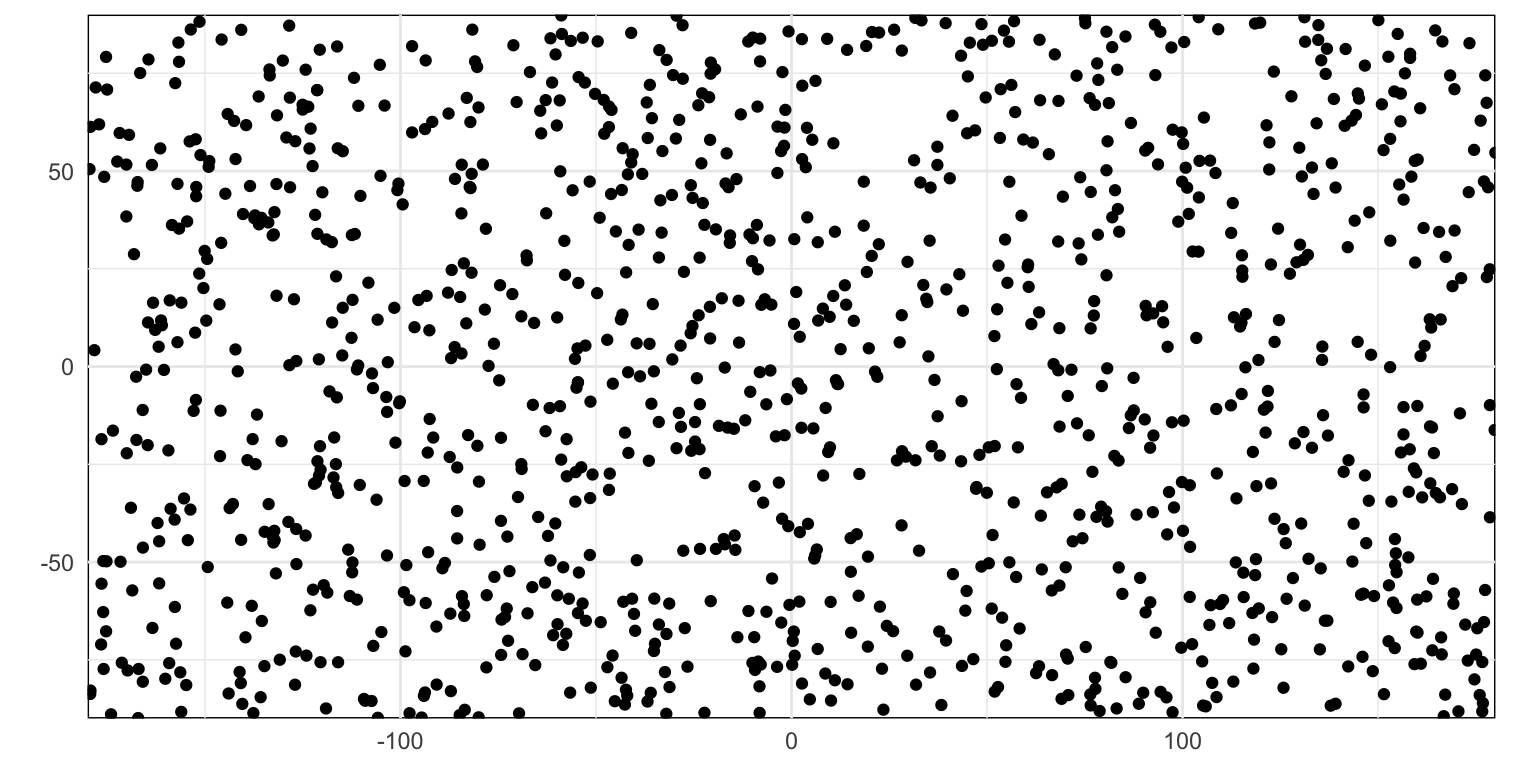
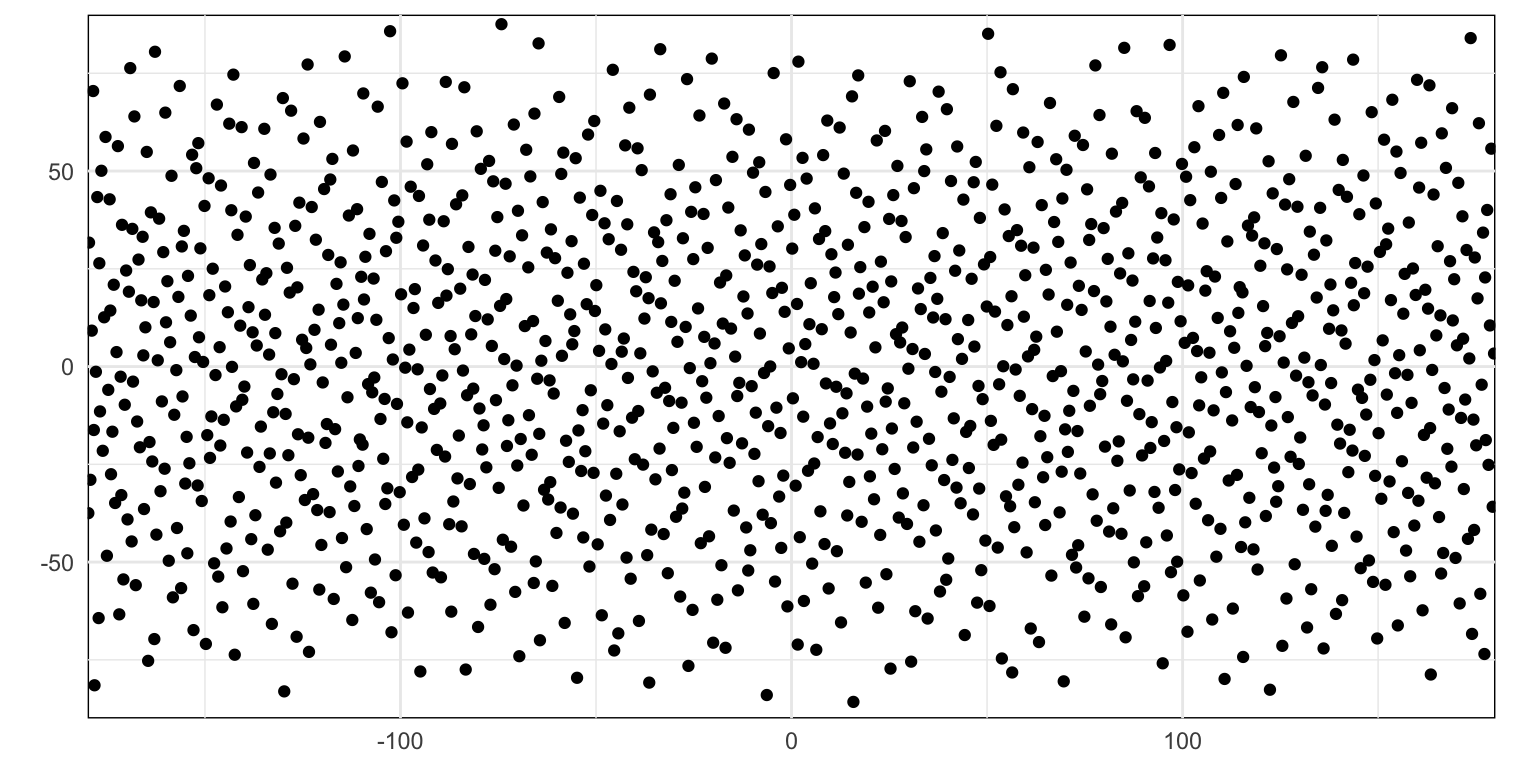
Figure 2: Simple uniform random pattern
Simple random pattern with a cosine correction for latitude
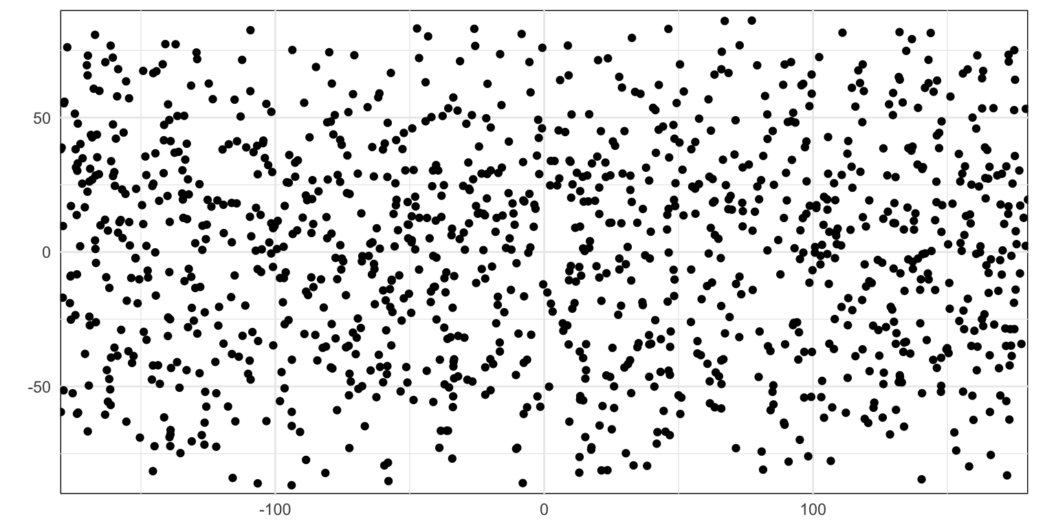
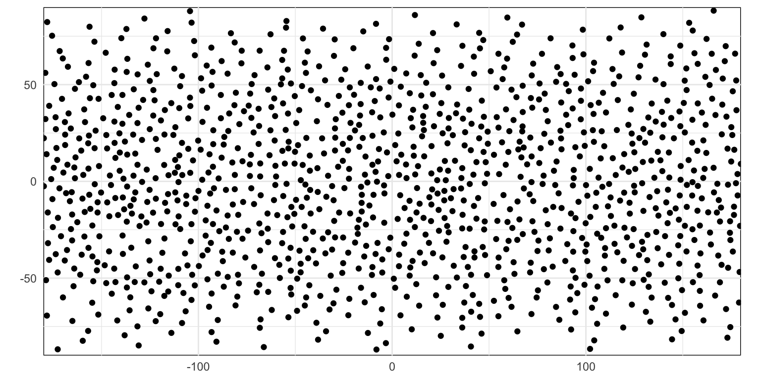
Next up the same pattern with the cosine correction from my earlier post.
pattern2 <-tibble(x =runif(n_points) *360-180,y =acos(runif(n_points, -1, 1)) / pi *180-90,generator ="Uniform random cosine-corrected")plot_pp(pattern2)
Figure 3: Uniform random pattern with cosine correction
In later patterns I have applied this cosine correction where the underlying process generates uniformly distributed y coordinates.
A pattern from a spatial point process
My first thought here was to use a sequential spatial inhibition process. This is a spatial point process where points are generated at random locations, but rejected if they are closer than some inhibition distance to an existing point already in the pattern. This is easily done in Euclidean space using the spatstat::rSSI function. In latitude-longitude space this won’t work because distances are not calculable using the Pythagorean function on coordinates.
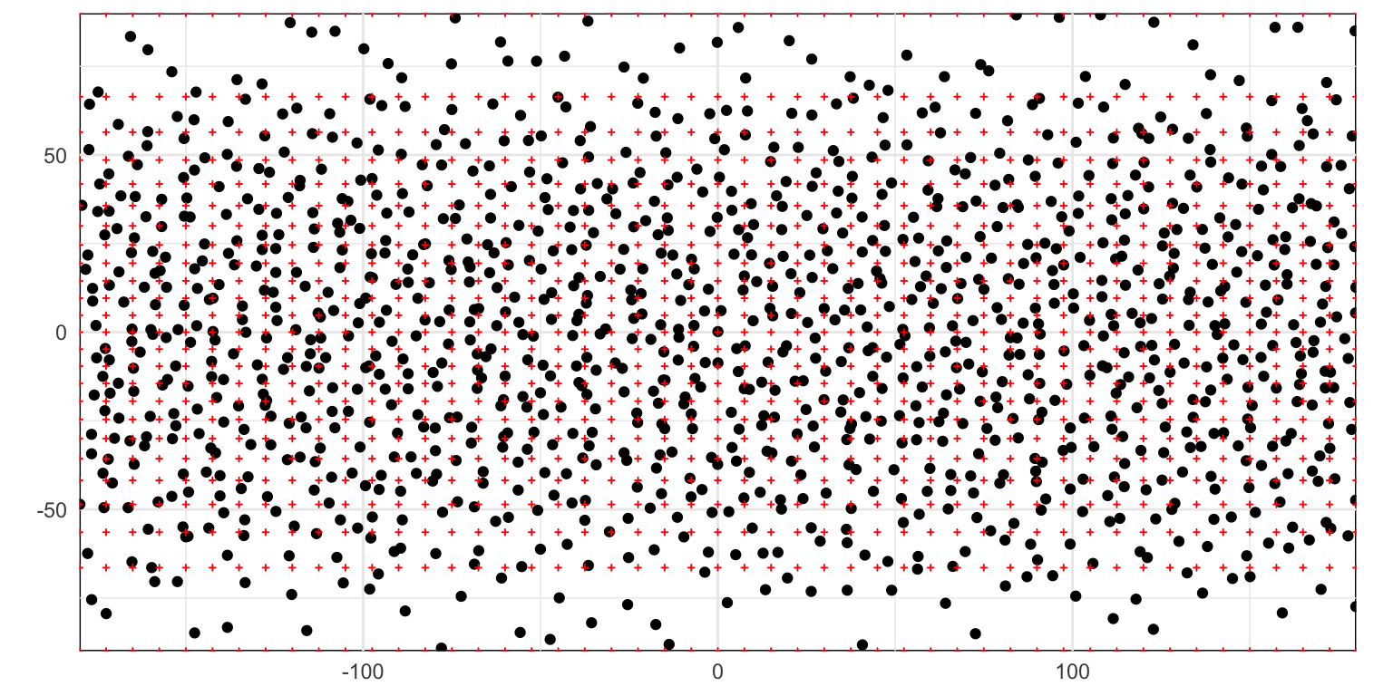
Instead, I have opted for the uniform point process (just as above), but specifying a tiling (a tessellation) of the space with approximately equal-area tiles. Using the formula for the y coordinate of a cylindrical equal-area projection \(y=sin\phi\), we can generate approximately equal-area rectangles in latitude-longitude space as below. I emphasise the approximation here, because it is only approximate. Rectangles in lat-lon space are not rectangles on the globe after all.
The number of gridlines we need in each direction is determined here.
2
x coordinates are trivially equally spaced.
3
y coordinates approximately equally spaced in the transformed space.
Figure 4: Stratified random point process
I’ve plotted the coordinates of the grid used to ‘thin’ the points at high latitudes for reference. The process generates only one point in each of these cells. However… the thinning is not continuous and there are a number of points very close to the poles, where of course the available area is zero!
Quasi-random sequences
These are the processes that were new to me, which showed up when I started looking for R packages that could do even sampling in 2D spaces. The first package to show up was spacefillr. This implements a number of such sequences, but we’ll look here at the Halton sequence, because its workings are relatively easy to understand, and the implementation in the spbal package provides more options.
:Halton sequences are generated using a pair of coprime numbers, i.e., two numbers with no common factors. The simplest example is 2 and 3. Each of the selected numbers specifies a sequence by repeated subdivision of the interval 0 to 1. So for 2 we get
Pairing these sequences gives us coordinates of points in the unit square. Different generating numbers can be chosen (provided they are coprime) and different starting points in each sequence can be paired, to give a wide variety of deterministically generated quasi-random patterns. The spbal package provides a highly configurable interface to generate such sequences using the cppRSHalton_br function. We can see the procedures inner workings clearly by examining the first few elements in the sequence:
These appear entirely regular, and some regularity is evident in the patterns generated (see Figure 5), although it is less apparent than might be anticipated on considering the numerical values alone. The main interest in Halton sequences is their desirable evenness of distribution for sampling purposes, which is apparent in Figure 5.
pattern4 <-cppRSHalton_br(n_points, bases =c(2, 3),seeds =c(14, 21))$pts |>as.data.frame() |>rename(x = V1, y = V2) |>mutate(x = x *360-180, y =acos(y *2-1) / pi *180-90,generator ="Halton")plot_pp(pattern4)
1
The coprime generating values.
2
The starting positions in the sequence for each generating value.
Figure 5: Points generated by a Halton sequence
Details concerning generation of Halton sequences and their statistical properties are provided by Faure and Lemieux.2
A ‘home-grown’ parameter-free pattern generator
Here I use a seemingly trivial (but not very efficient!) algorithm to generate some home-made evenly distributed points, without the need to specify any (spatial) parameter like the inhibition distance required by rSSI. I found the inspiration for this in this detailed blog post about generating :blue noise, which was in turn based on an algorithm described by Mitchell.3
Matters are complicated by having to calculate distances in latitude-longitude space, which we do using the :Haversine formula
for the distance between two lon-lat locations\(\left(\lambda_1,\varphi_1\right)\) and \(\left(\lambda_2,\varphi_2\right)\), although because we only need the relative distances we don’t use the \(2r\) scaling. The need to calculate toroidal distances described in the blogpost is obviated by calculating distances on the sphere which wraps in a similar way.
The simple idea of this algorithm is that each time we add a new point we generate a set of points (candidates) to choose from, and select the one with the largest minimum distance to an existing point in the pattern. Making the algorithm more efficient would involve only checking the distance to points known to be close to candidate points using some kind of spatial index or binning structure.
I use the outer function to do all pairwise differences and products of data in the two supplied matrices more efficiently than by nested loops.
2
The choice_scaling parameter determines how rapidly the number of candidate points grows with the size of the existing data set. It should be strictly greater than 1 or no points will ever get added! Including a log factor stops the speed of the algorithm from falling too rapidly as points are added.
3
The apply(1, min) operation finds the smallest distance in each row (i.e. distance to nearest neighbour in the existing set of points), and which.max() identifies the row with the largest minimum distance.
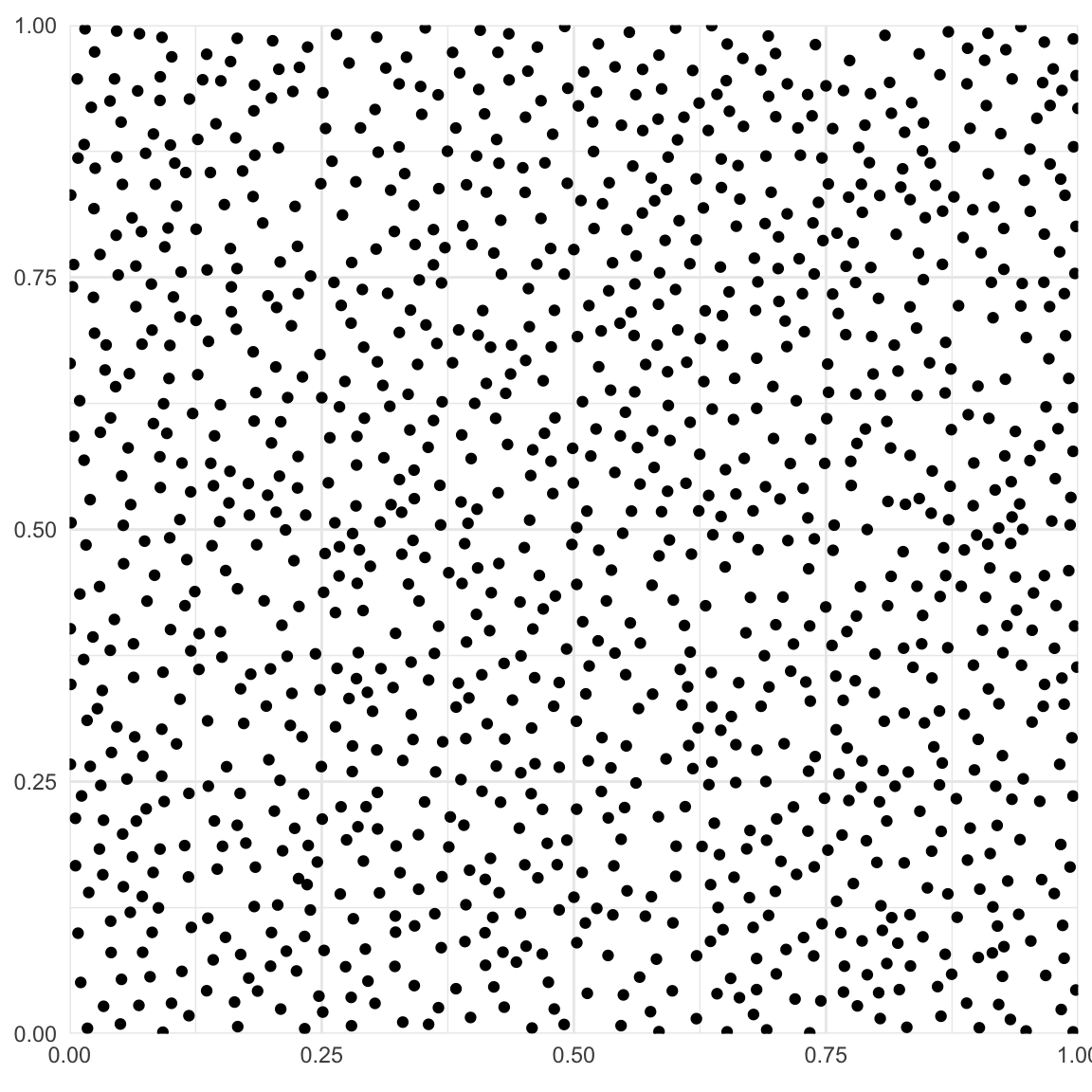
Figure 6: A pattern generated using a ‘blue noise’ algorithm by iteratively choosing the most remote random additional point among a set of choices
Putting all these points on the globe
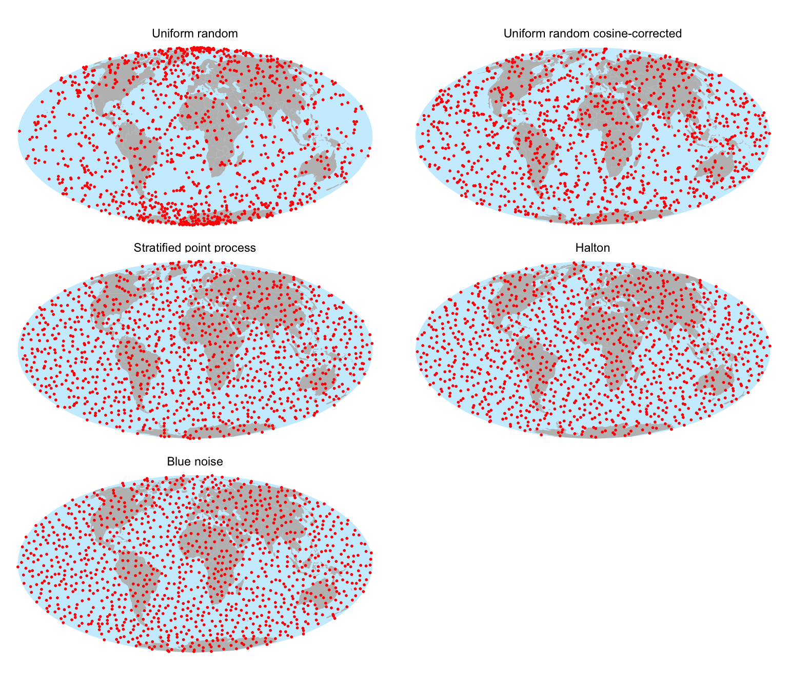
We now apply a transformation from the lat-lon Cartesian coordinates to the globe that is equal-area as shown in the previous post. We can combine all the points into a single data set and use facet_wrap for side-by-side comparison.
Figure 7: Side-by-side comparison of five patterns projected onto the globe
With the obvious exception of the uniform random pattern, which exhibits definite clumping, all of these seem to do a reasonable job of producing a random arrangement of points evenly distributed over the globe.
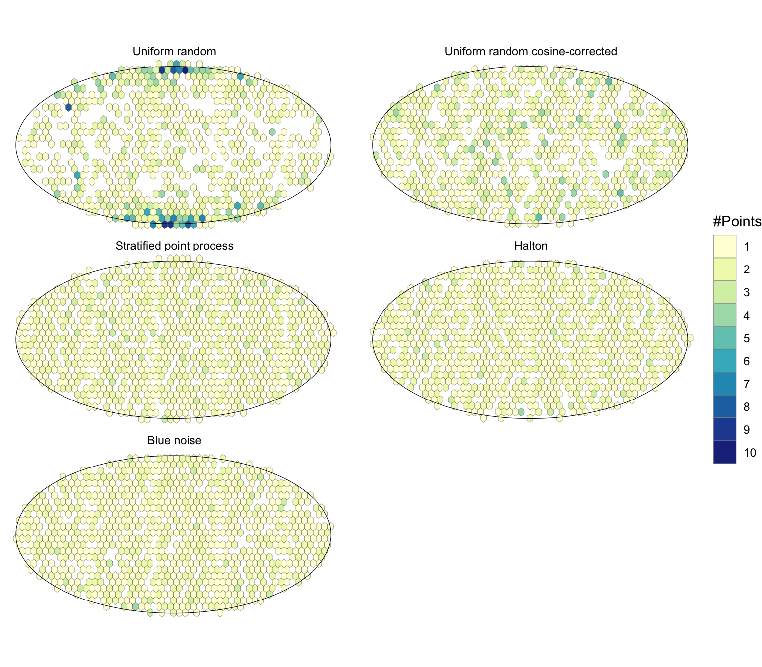
From the perspective of avoiding clumping we can try to make the comparison slightly more precise by making hexbin density plots of the points.
xy <- all_points |>st_coordinates() |>as.data.frame() |>bind_cols(all_points)nx <-sqrt(n_points / pi) *2*sqrt(aspect_ratio)ny <- nx *2/sqrt(3) /sqrt(aspect_ratio)ggplot(xy) +geom_hex(aes(x = X, y = Y, fill =as.factor(after_stat(count))), bins =c(nx, ny), linewidth =0.1, colour ="#666666") +scale_fill_manual(values =c4a("brewer.yl_gn_bu", 11),breaks =1:10, guide ="legend", name ="#Points") +annotate(geom ="path", x = x, y = y, linewidth =0.2) +coord_equal() +facet_wrap( ~ generator, ncol =2) +theme_void()
1
ggplot2::geom_hex insists that the point counts are ‘continuous’ which is what forces me to convert at a factor, so that I can use a legend not a colour ramp here. Another instance of ggplot2’s strong preference for not classing data, see this recent post in the context of choropleth maps.
Figure 8: Side-by-side comparison of hexbin density plots of the five point patterns
The uniform random pattern clearly exhibits the most uneven distribution of points. The cosine-corrected version is better although there is still unevenness in the mid-latitudes, as we would expect because there is no interaction between points in the pattern: the presence of a previous point does not block another point showing up close by. The stratified point process and Halton patterns are better again. The latter of these is particularly surprising, given its completely deterministic generative process.
Somewhat to my surprise my ‘homebrew’ blue noise compares well with the other four patterns for evenness of distribution. This is particularly nice given that it requires no spatial parameter to be supplied, only one that (perhaps only marginally) affects the quality of the patterns produced.
Final thoughts
It is intriguing to me that blue noise is seemingly not a standard spatial point process. Unlike sequential spatial inhibition to which it is similar it requires no spatial parameter to be tuned to get a desired result, and it cannot fail to produce the requested number of points. It is also a reasonable plausible process from a ‘mechanism’ perspective. Imagine for example retailers considering premises in which to set up shop and examining a number of different sites, then choosing the one farthest from any potential competitor. It’s at least as compelling in that respect as a model of the outcome of competition between event locations as SSI.
Since it seems useful, I provided some ‘hooks’ in the implementation above to allow use of different distance functions and ‘windows’ for point generation. Here’s an example in a simple Euclidean space, using :Manhattan distance to determine the best new point among candidates.
Having said that, the circular game board eventually led me to generate the patterns in NetLogo by randomly displacing each new flower from the centre of the circle by a random distance in a random direction, and retrying until they were no closer to another flower than some set distance.↩︎