Code
library(sf)
library(tidyr)
library(dplyr)
library(patchwork)
library(ggplot2)
library(sfnetworks)
library(tidygraph)
library(raybevel)
library(rmapshaper)
library(spatstat)
library(terra)

theme_set(theme_void())In this post and this one I covered various GIS transformations from respectively points and lines. Here, we carry on down this path with some of the transformations available when your geospatial data consist of areas.
As it turns out, area data are complicated, and some of the associated transformations have more than a few wrinkles, so one post has become two, and this post only covers polygons → points, and polygons → lines.1
As will become clear, that’s more than enough to be going on with. Check out the number of packages imported below, if you’re not convinced.
library(sf)
library(tidyr)
library(dplyr)
library(patchwork)
library(ggplot2)
library(sfnetworks)
library(tidygraph)
library(raybevel)
library(rmapshaper)
library(spatstat)
library(terra)
theme_set(theme_void())As always, we need some data. This time it’s useful to have data with associated attributes, so we’ll use some real data, conveniently to hand, namely New Zealand 2018 census Statistical Areas, with populations.
polygons <- st_read("sa2-generalised.gpkg")
polygon1 <- (polygons |>
st_cast("POLYGON"))$geom[1]
polygon2 <- (polygons |>
filter(SA22018_V1_00_NAME == "Mangatainoka"))$geom[1]
wellington <- polygons |>
filter(TA2018_V1_00_NAME == "Wellington City") |>
select(population)And here are what those look like. The two single polygons have been picked out for their complexity, and in the case of the second one, for its having a couple of holes, which makes some transformations trickier.
g1 <- ggplot() +
  geom_sf(data = wellington, aes(fill = population)) +
  scale_fill_distiller(palette = "Reds") +
  guides(fill = "none") +
  ggtitle("Wellington")
g2 <- ggplot(polygon1) + geom_sf() + ggtitle("Polygon #1")
g3 <- ggplot(polygon2) + geom_sf() + ggtitle("Mangatainoka")

g1 | g2 | g3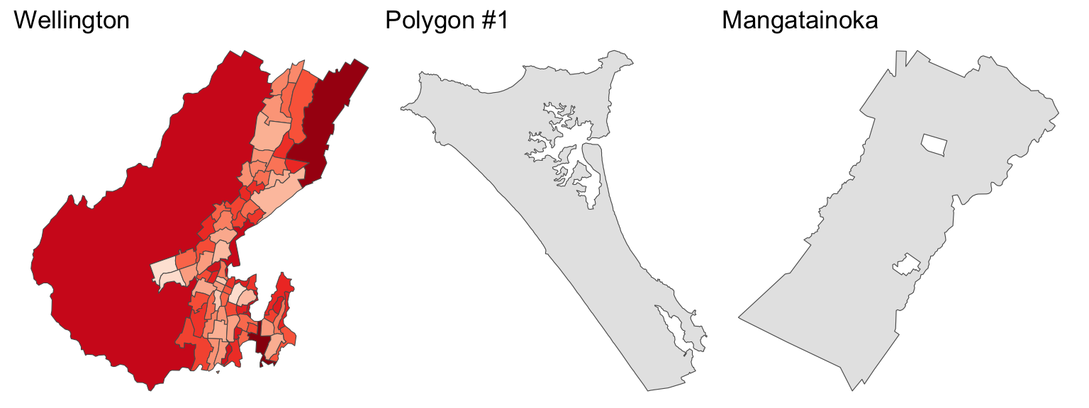
The table of transformations™ calls for ‘Centroid’, which is easily accomplished with the st_centroid function.
centroids <- wellington |>
  st_centroid()

ggplot() +
  geom_sf(data = wellington) +
  geom_sf(data = centroids)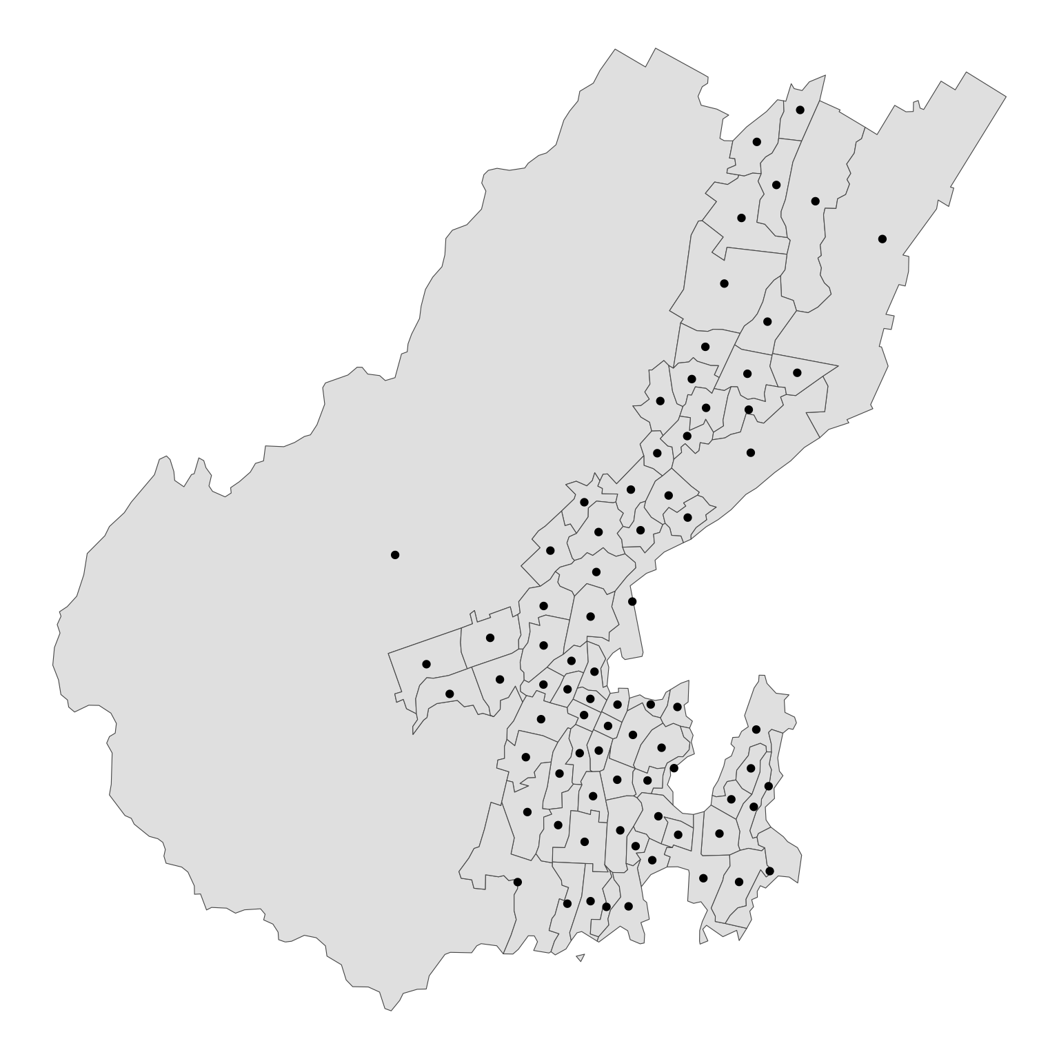
As is likely well-known, the centroid of an area is not guaranteed to be inside the area. There are a couple of examples of that in these data. A function that returns a point guaranteed to be inside the area is st_point_on_surface and this should be used in preference to st_centroid when the point2 is to enable data to be reliably joined between different polygon layers—say, for example, a set of polygons, and a set of the ‘same’ polygons which have been simplified or generalised.
The difference is shown in the figure below.
polygons_with_no_centroid <- wellington |>
  slice(((wellington |>
            st_contains(centroids) |>
            lengths()) == 0) |> which())

bb <- st_bbox(polygons_with_no_centroid)

points_on_surface <- polygons_with_no_centroid |>
  st_point_on_surface()

ggplot() +
  geom_sf(data = wellington, fill = "lightgrey") +
  geom_sf(data = polygons_with_no_centroid,
          colour = "pink", lwd = 1) +
  geom_sf(data = centroids) +
  geom_sf(data = points_on_surface, colour = "red") +
  coord_sf(xlim = bb[c(1, 3)], ylim = bb[c(2, 4)])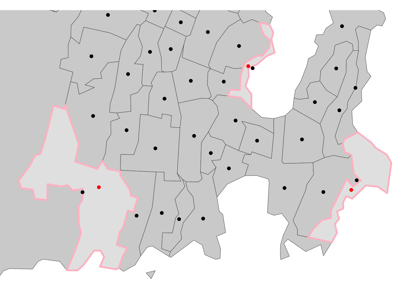
This case is relatively simple, insofar as the polygons that do not contain a centroid have not ‘acquired’ one from a neighbour, so checking for zero centroids correctly identifies ‘problem’ polygons.
It is easy to imagine this not working, however. For example, two intertwined U-shaped polygons, can ‘swap’ centroids, as shown below. If you were to use these centroids to move data between layers then the data associated with these polygons would get swapped in the process.
square <- function(dx, dy) {
  (st_linestring(
    matrix(c(0, 0, 1, 1, 0,
             0, 1, 1, 0, 0), ncol = 2)
  ) + c(dx, dy)) |>
    st_cast("POLYGON")
}

u_polygons <-
  mapply(square,
         dx = rep(0:3, 4),
         dy = rep(3:0, each = 4),
         SIMPLIFY = FALSE) |>
  st_sfc() |>
  data.frame() |>
  st_sf(crs = 2193) |>
  mutate(
    ID = as.factor(c(1, 1, 1, 1,
                     1, 2, 2, 2,
                     1, 1, 1, 2,
                     2, 2, 2, 2))) |>
  group_by(ID) |>
  summarise() |>
  mutate(geometry = st_simplify(geometry, dTolerance = 1e-6))

us_centroids <- u_polygons |> st_centroid()

ggplot() +
  geom_sf(data = u_polygons) +
  geom_sf_label(data = u_polygons, aes(label = ID)) +
  geom_sf(data = us_centroids) +
  geom_sf_label(data = us_centroids, aes(label = ID), colour = "red")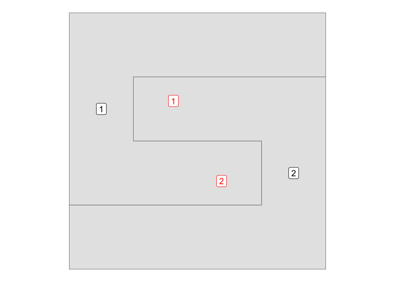
TL;DR: be careful using centroids as a convenient way to summarise the location of polygons!
The straight skeleton of a polygon is the set of lines that it collapses down along as it is negatively buffered and eventually disappears. We can see how this works for a simple convex shape without too much trouble.
shape <- st_polygon(
    list(matrix(c(0, 0, 1, 2, 2, 1, 0,
                  0, 1, 2, 2, 1, 0, 0), ncol = 2))) |>
  st_sfc(crs = 2193)

collapsed_polys <-
  mapply(st_buffer, shape, dist = -(0:7/10), nQuadSegs = 0,
    SIMPLIFY = FALSE) |>
  st_sfc()

ggplot() +
  geom_sf(data = collapsed_polys, fill = NA)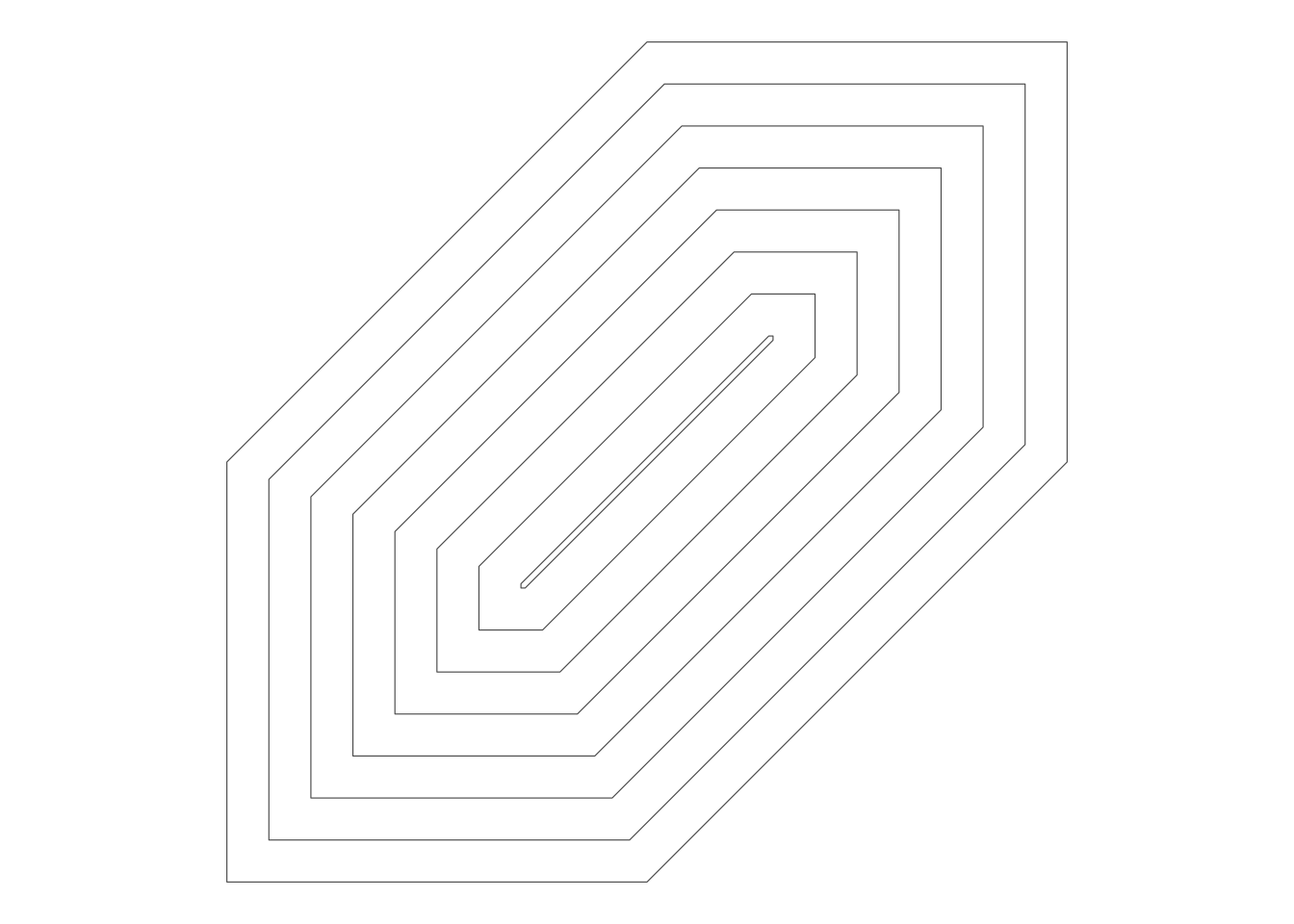
Unsurprisingly, things get complicated quickly when we move away from simple convex shapes, especially when we add the additional complication of holes. Sadly, there is no st_skeleton function in sf. Happily, this being R, there’s a package for that™. raybevel is a package for generating straight skeletons including extensions into 3D and roof models. If you squint at the simple example, you can see the relevance of roof models to this topic. In fact, according to wikipedia, this is the context in which the straight skeleton of a polygon first appeared as far back as 1877. The picture below (snipped from a recent property listing in Wellington reinforces this point.

The raybevel::skeletonize function meets our requirements. The result from that function is a collection of points, and collection of source-destination pairs of point ids, which we can link to one another to create the skeleton. The sfnetworks package is a good way to do the linking to make the result into a sf dataset.
sk <- st_coordinates(shape)[, 1:2] |>
  skeletonize()

nw <- sfnetwork(sk$nodes |> st_as_sf(coords = 2:3),
                edges = sk$links |> filter(edge == FALSE),
                directed = FALSE,
                node_key = "id",
                edges_as_lines = TRUE)

ggplot() +
  geom_sf(data = shape) +
  geom_sf(data = nw |> st_as_sf("edges") |>
            st_set_crs(2193), colour = "red", lwd = 0.2)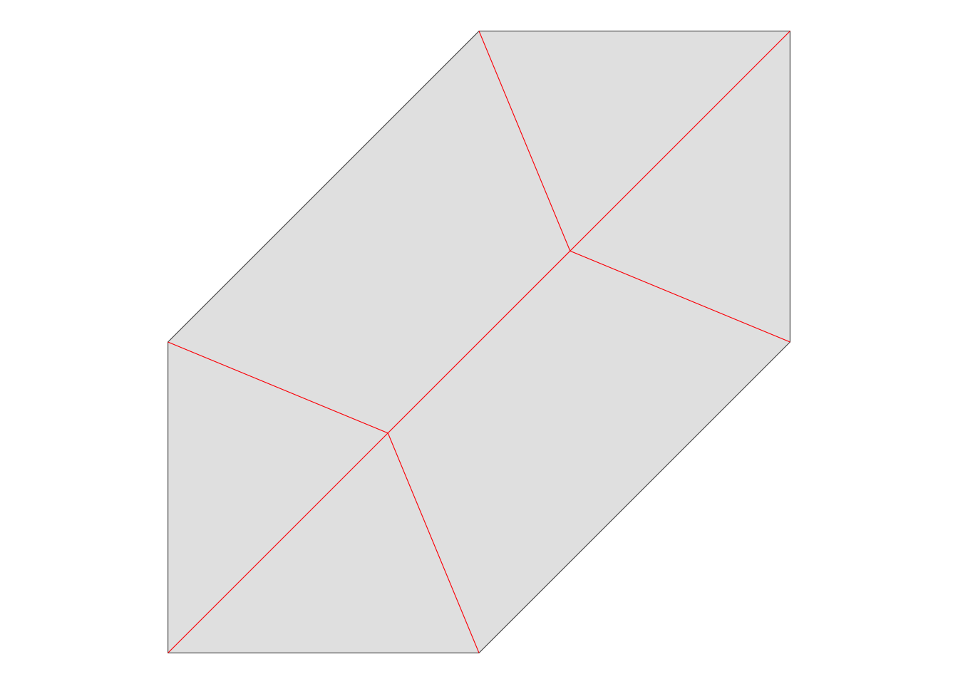
Here is a more taxing example:
sk <- st_coordinates(polygon1)[, 1:2] |>
  skeletonize()

nw <- sfnetwork(sk$nodes |> st_as_sf(coords = 2:3),
                edges = sk$links |> filter(edge == FALSE),
                directed = FALSE,
                node_key = "id",
                edges_as_lines = TRUE)

g1 <- ggplot() +
  geom_sf(data = polygon1) +
  geom_sf(data = nw |> st_as_sf("edges") |>
            st_set_crs(2193), colour = "red", lwd = 0.2)
g1
If we need to handle holes in the polygon, we have to also supply skeletonize with a list of the hole polygons, which requires us to do a bit more work:
exterior <- polygon2 |>
st_exterior_ring()
holes <- exterior |>
st_difference(polygon2) |>
st_cast("POLYGON")
xy <- st_coordinates(exterior)[, 1:2]
xy_holes <- holes |>
lapply(st_coordinates) |>
lapply(subset, select = 1:2)
sk <- skeletonize(xy, xy_holes)st_coordinates produces additional columns that skeletonize will choke on if we don’t remove them.
After that the further steps required are the same as before and the resulting skeleton is shown below.
nodes <- sk$nodes |> st_as_sf(coords = 2:3)
edges <- sk$links |> rename(from = source, to = destination)

nw <- sfnetwork(nodes,
                edges = edges |> filter(edge == FALSE),
                directed = FALSE,
                node_key = "id",
                edges_as_lines = TRUE)

ggplot() +
  geom_sf(data = polygon2) +
  geom_sf(data = nw |> st_as_sf("edges") |>
            st_set_crs(2193), colour = "red", lwd = 0.2)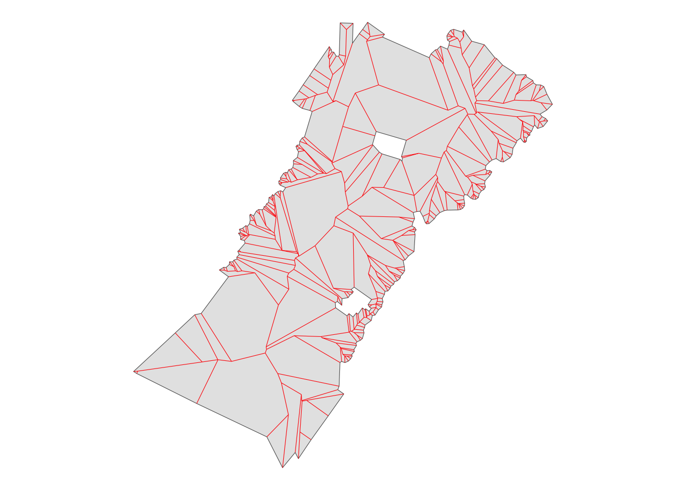
While I am here, I might as well show the related medial axis, which is the set of points in a polygon that have two or more equidistant closest points on the polygon boundary. Perhaps the most obvious example where this might be of interest is tracing a possible centre-line of a river.
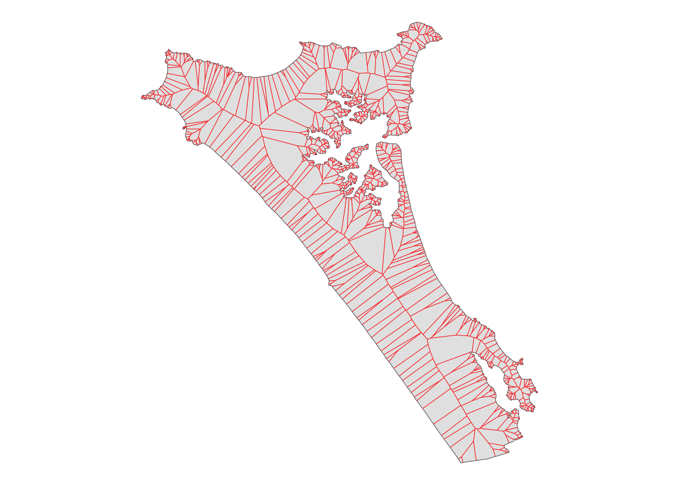
The medial axis of a polygon can be approximated as the edges of the Voronoi tessellation of the polygon vertices.
bb <- polygon1 |> st_buffer(1000) |> st_bbox() |> st_as_sfc()
medial_axis <- polygon1 |>
st_union() |>
st_cast("MULTIPOINT") |>
st_voronoi() |>
st_cast() |>
st_intersection(bb) |>
rmapshaper::ms_lines() |>
st_intersection(polygon1) |>
data.frame() |>
st_sf() |>
filter(st_geometry_type(geometry) == "LINESTRING" |
st_geometry_type(geometry) == "MULTILINESTRING")
g2 <- ggplot() +
geom_sf(data = polygon1) +
geom_sf(data = medial_axis, colour = "red", lwd = 0.2) +
ggtitle("Medial axis")
g1 + ggtitle("Straight skeleton") | g2st_intersection step produces a jumble of geometry types including points, and multipoints, so this filter step removes those.
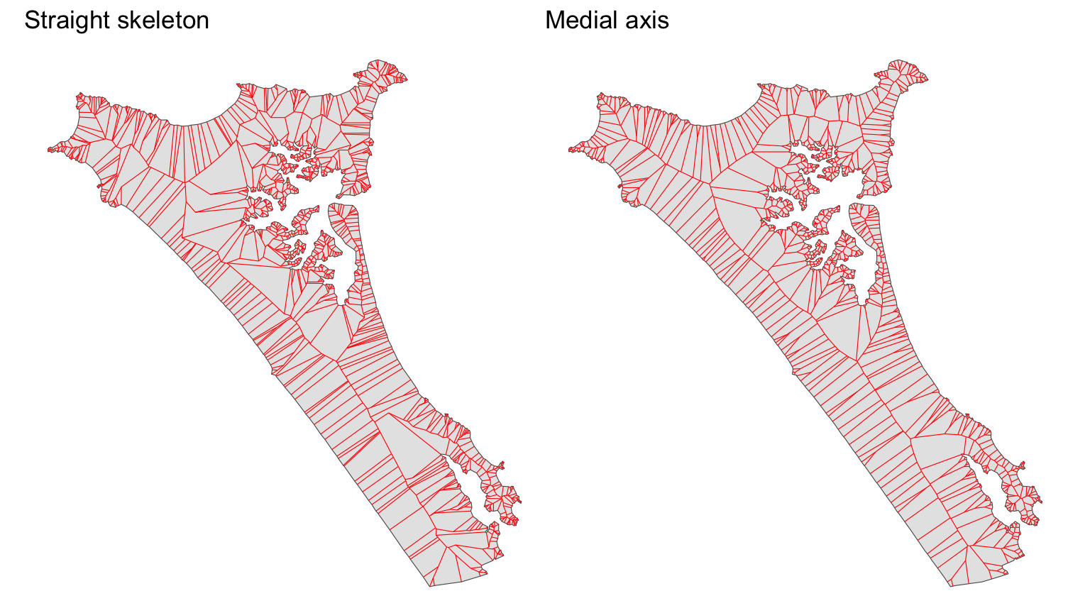
Because the sf::st_voronoi function produces a set of polygons, we have to convert these to a set of lines, which is most conveniently accomplished via the rmapshaper::ms_lines function. Even so, there’s still a need for several st_cast steps along the way, which doesn’t make for the cleanest code.
Perhaps surprisingly, a cleaner, less confusing sequence of operations uses the dirichletEdges function in spatstat to get the same result.3
xy <- polygon1 |>
st_sf() |>
st_cast("POINT") |>
slice(-1) |>
st_coordinates()
pp <- ppp(xy[, 1], xy[, 2], as.owin(bb))
edges <- dirichletEdges(pp) |>
st_as_sf() |>
filter(label == "segment") |>
select(-label) |>
st_set_crs(2193) |>
st_intersection(polygon1)
ggplot() +
geom_sf(data = polygon1) +
geom_sf(data = edges, colour = "red", lwd = 0.2)spatstat point patterns.
spatstat point pattern from our polygon coordinates.
spatstat
Both these results, because they are based only on the vertices of the polygon are only approximations to the true medial axis, which should be derived from the Voronoi diagram of the polygon’s edges. Such diagrams may contain segments that are parabolic arcs, and not only straight line segments as is the case for a Voronoi diagram derived from point data. You can get some feel for the complexities that might be involved in the precise calculation from this post of mine, and from this blog post by a computational geometer who knows what they are doing.
I mentioned that the distance surface in the lines → fields section of the previous post might contain ‘spoilers’ for polygon skeletons. This wasn’t quite correct. However there’s certainly a way to derive the medial axis of a polygon by going via a line distance surface.
Here’s the code, which is adapted from that previous post. The additional step of deriving a slope layer from the distance surface helps to illustrate the relationship even more clearly.
target_raster <- polygon1 |>
  as("SpatVector") |>
  rast(res = 100)

target_points <- target_raster |>
  as.points() |>
  st_as_sf()

d1 <- target_points |>
  mutate(
    distance = st_distance(geometry, polygon1 |> st_cast("LINESTRING")) |>
      apply(MARGIN = 1, min)) |>
  as("SpatVector") |>
  rasterize(target_raster, field = "distance") |>
  mask(polygon1 |> as("SpatVector"))

d2 <- d1 |> terrain(neighbors = 4)

names(d1) <- "z"
names(d2) <- "z"g1 <- ggplot() +
geom_raster(
data = d1 |> as.data.frame(xy = TRUE),
aes(x = x, y = y, fill = z)) +
geom_sf(data = polygon1, fill = NA) +
scale_fill_viridis_c(option = "B", direction = -1) +
guides(fill = "none") +
ggtitle("Distance surface")
g2 <- ggplot() +
geom_raster(
data = d2 |> as.data.frame(xy = TRUE),
aes(x = x, y = y, fill = z)) +
geom_sf(data = polygon1, fill = NA) +
scale_fill_viridis_c(option = "B") +
guides(fill = "none") +
ggtitle("Distance surface slope")
g1 | g2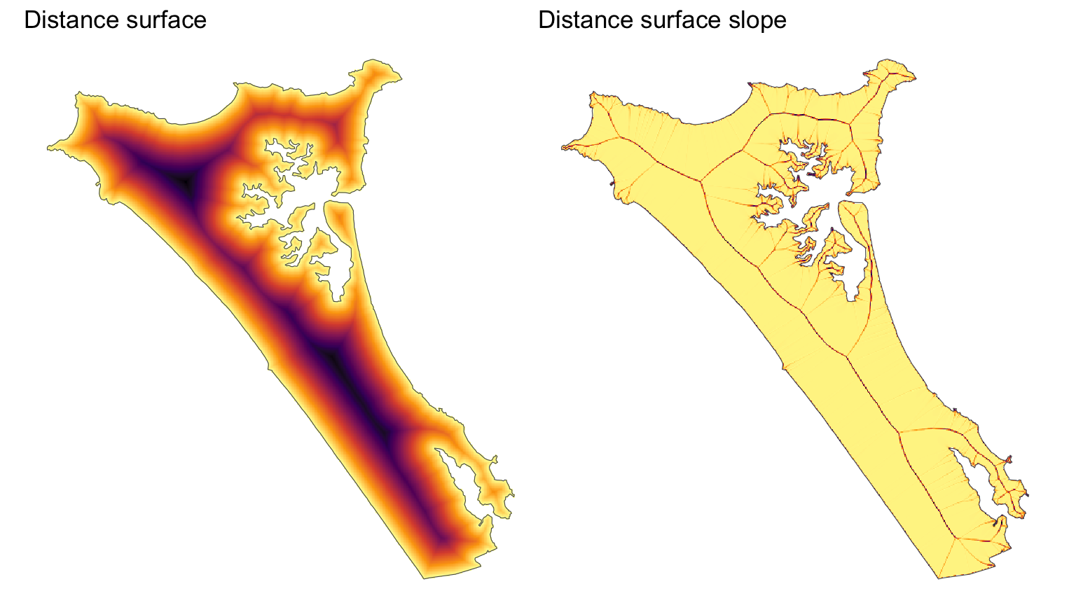
And here they are plotted together showing the expected match.
g1 + geom_sf(data = medial_axis, colour = "white", lwd = 0.2)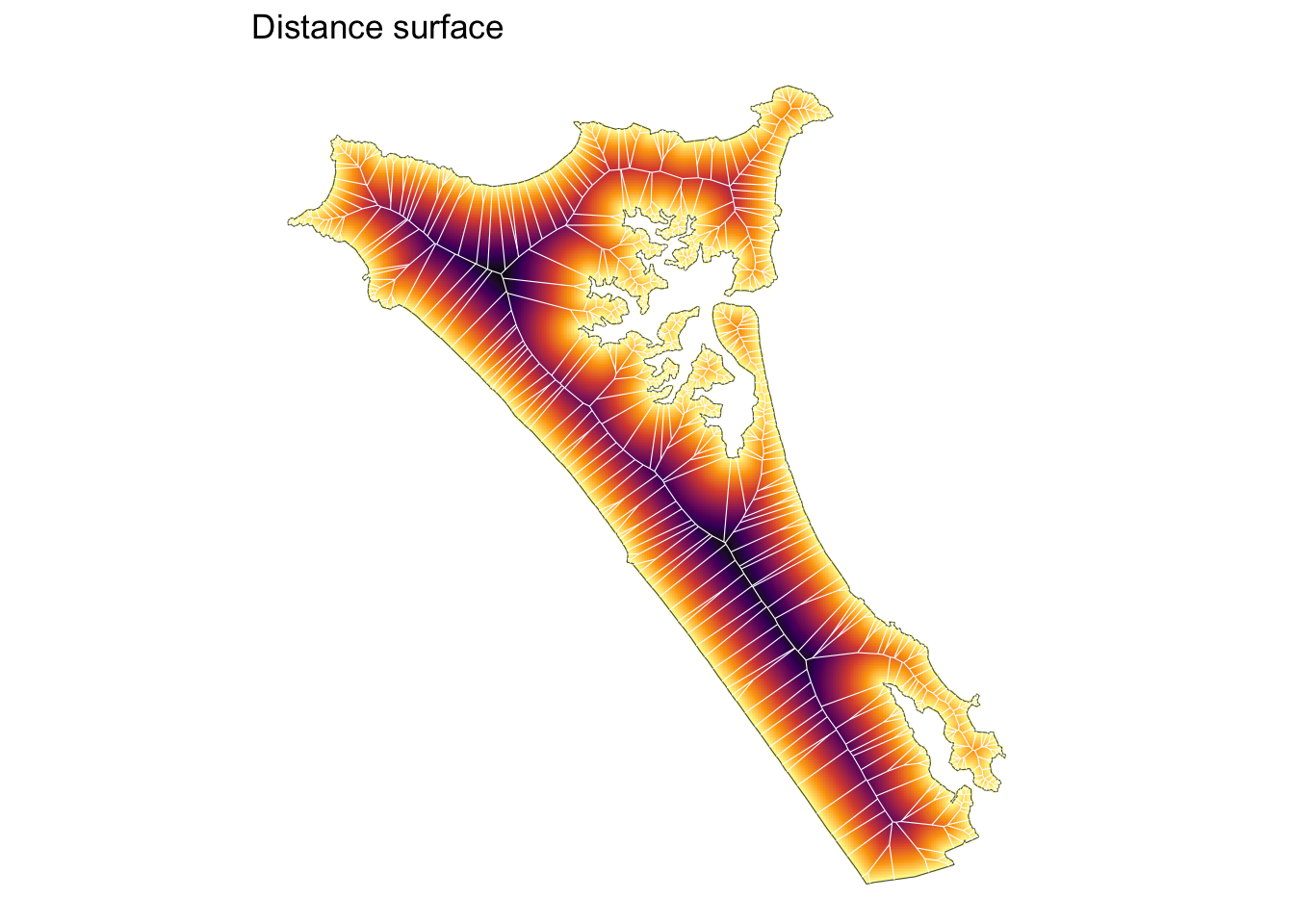
Calculated at sufficient precision this raster approach may be a more useful way to find the medial axis.
The transformations of area objects, particularly to lines, led down deeper rabbit holes than expected, so that’s it for now. Tune in again soon for transformations to areas and to fields.
![]()