A process for building a hierarchical partition of a gridded population dataset
geospatial
R
tutorial
aotearoa
population
cartography
Author
David O’Sullivan
Published
June 20, 2025
In a recent post I developed some R code to quadrisect the population of Aotearoa New Zealand. At the end of that post I airily suggested
that lurking in here are almost certainly the ingredients for a treemap/quad-tree approach to cartograms
The thought was something like, bisect the population data (by population), then bisect each half, then bisect each quarter and so on. The bisection procedure using weighted medians was thoroughly explored in the earlier post.
Now, as promised, here’s that iterative bisection process, which yields something like a population quadtree. Each leaf of the tree accounts for some power-of-two fraction of the population (in the example below 1/1024th). If we had the location of every individual in the data as a point, the result is roughly what we would get if we were adding those points to a binary space partition data structure.
It would be nice to do this as a quad-tree where at each step we subdivide the population into 4 more or less equal groups, but that would require allowing the lines subdividing the space to be at arbitrary angles at each step and would demand much more complicated coding than what follows. Sticking to halving the population at each step means we can work with only east-west or north-south bisectors and simplifies matters greatly. I’ll set the more complicated quad-tree approach to one side for now.
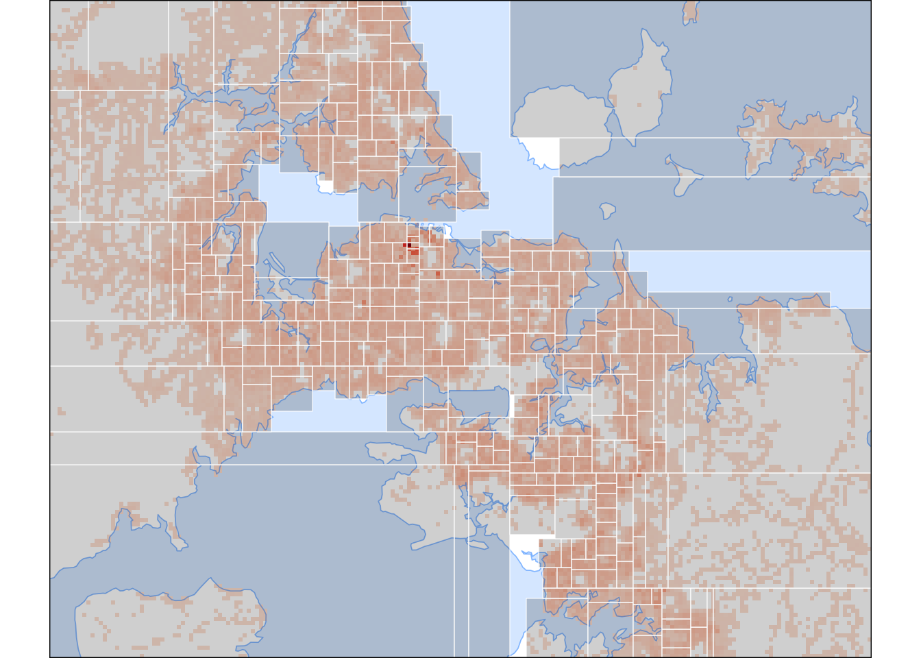
As an indication of where we are going, here’s the end result, showing approximately equal population rectangular areas around Christchurch.
Figure 1: A zoomed in map of the Christchurch area.
Preliminaries
As usual, we need some libraries and data.
Code
library(sf)library(dplyr)library(stringr)library(ggplot2)library(tmap)library(spatstat) # for weighted median functionlibrary(data.tree) # to build a treepop <-read.csv("nz-pop-grid-250m.csv") |> dplyr::filter(x <2.2e6)nz <-st_read("nz.gpkg")
1
This is to remove the far-flung Chatham Islands, which in this case detract from the pattern of the quadtree.
A useful helper functions is get_rectangle() to return a sf polygon based on x and y limits.
A convenience function to get an sf polygon given x and y limits.
Iterative population bisection
Central to this whole exercise is a function that given a dataframe of x, y, and population data, along with a bounding extent, returns two rectangles within the extent, each containing half the population. This is accomplished using a weighted median as in the previous post. Because we are working only with north-south or east-west subdivisions there isn’t any especially complicated geometry needed to handle this.
Code
split_population <-function(pop_pts, bounds) { w <- bounds[1]; e <- bounds[3]; s <- bounds[2]; n <- bounds[4]; width <- e - w; height <- n - s; xy <- pop_pts |>filter(x > w, x <= e, y > s, y <= n) bbs <-list()if (height > width) { # cut east-west at median y my <-weighted.median(xy$y, xy$pop_250m_grid) south <- xy |>filter(y <= my) x1 <-min(south$x) -125; x2 <-max(south$x) +125; y1 <-min(south$y) -125; y2 <- my; bbs[[1]] <-get_rectangle(x1, y1, x2, my) north <- xy |>filter(y > my) x1 <-min(north$x) -125; x2 <-max(north$x) +125; y1 <- my; y2 <-max(north$y) +125; bbs[[2]] <-get_rectangle(x1, my, x2, y2) } else { # cut north-south at median x mx <-weighted.median(xy$x, xy$pop_250m_grid) west <- xy |>filter(x <= mx) x1 <-min(west$x) -125; x2 <- mx; y1 <-min(west$y) -125; y2 <-max(west$y) +125; bbs[[1]] <-get_rectangle(x1, y1, mx, y2) east <- xy |>filter(x > mx) x1 <- mx; x2 <-max(east$x) +125; y1 <-min(east$y) -125; y2 <-max(east$y) +125; bbs[[2]] <-get_rectangle(mx, y1, x2, y2) } bbs}
1
Unpack the bounding box to west, east, bottom, and top values, and use these to get width w and height h.
2
We are only interested in the population inside the bounding box.
3
If the area is taller than it is wide, then cut east-west at the weighted median y coordinate, otherwise cut north-south at the weighted median x coordinate.
4
Here, and elsewhere the 125 offsets account for the fact that the grid cells are 250m, but we are using their central coordinates.
The bisection runs east-west if the extent of the bounding area is longer north-south than east-west, and will run north-south otherwise. This is to promote ‘squarer’ rectangles as outputs, although as we’ll see the vagaries of population distribution mean that plenty of long skinny rectangles make it through the process.
Using this splitter function it is straightforward to iteratively subdivide the data into halves by population to some requested depth. I found an R package data.tree that means I can store the results of an iterative splitting process like this as a tree, or more accurately as a linked set of ‘nodes’ with associated attributes. As is often the case in R, when a data structure that is not tabular appears the syntax is a little weird1, so figuring out how to use it took some experimentation. The Node$new() and using $ to invoke methods on objects was new to me, but I figured it out in the end.
Having struggled a bit to get data.tree working,2 the reward is nice compact code, which much more clearly expresses the intent to create a tree structure than some earlier sprawling and rather kludge-y list-based code.
The ‘root’ node which we call ‘X’ which has as its ‘bb’ attribute, a bounding box of all the population data.
2
Then, we repeatedly split the ‘leaf’ nodes of the tree in two, adding them to each leaf as child nodes.
A minor difficulty once the tree has been constructed is to retrieve the sf geometries intact. Because sf geometries are thinly wrapped R matrices and lists, they are prone to ‘reverting to type’ when you include them in R lists or other containers. Using data.tree the polygons did indeed revert to matrices, but it’s not difficult to retrieve them as polygons, which we do in the code below to assemble final simple feature datasets for mapping.
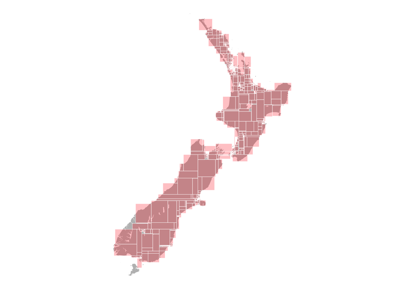
Figure 2: All 1024 cells at level 11 of the partition.
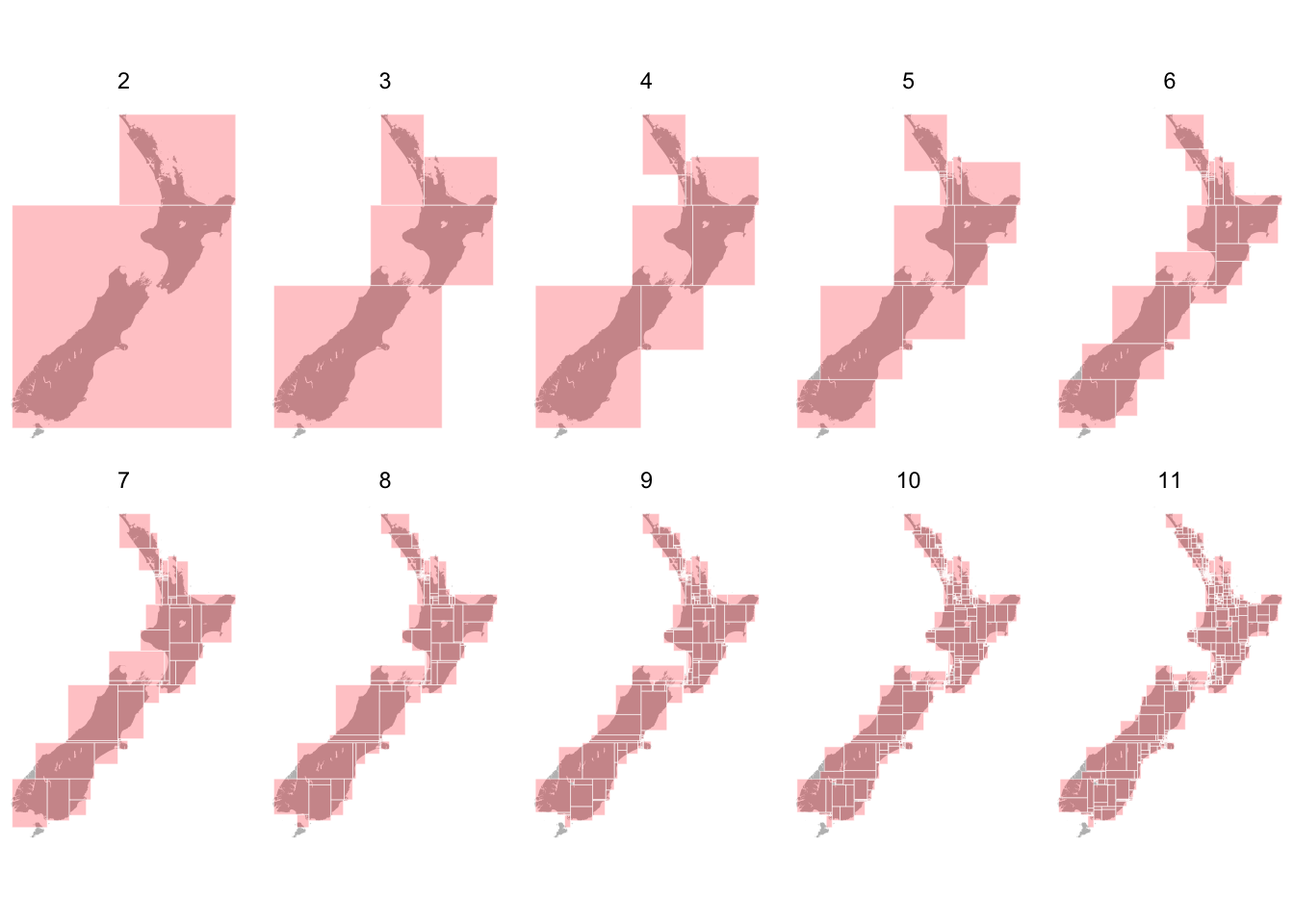
It’s also interesting to see the stages along the way to the final subdivision, which is conveniently done using a facet_wrap based on the level attribute in the all_levels dataframe
Figure 3: The sequence of bisections along the way to 1024 rectangles.
A close up look
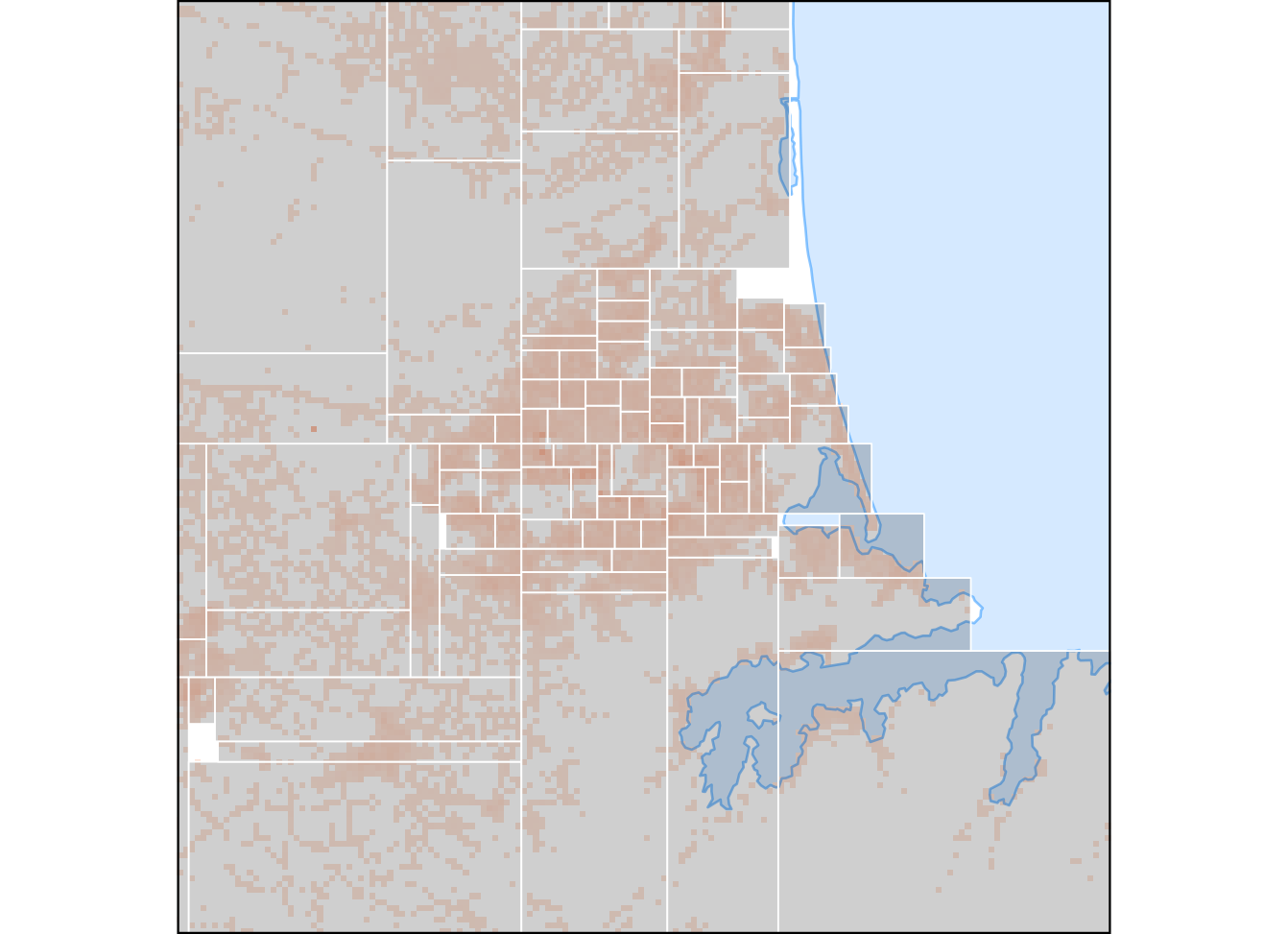
It’s also useful to look at a zoomed in local areas. As I’ve noted previously a big chunk of the country’s population is in Auckland, so it’s perhaps most interesting to look there. What emerges is a picture over an extended area3 of relatively evenly distributed population everywhere that is inhabitated (all the pink areas of the map), except for a concentration in a tiny area of the downtown centre. The result in terms of the space partition is relatively equal-sized areas across much of the populated suburban sprawl.4
Code
bb <-c(1.735e6, 5.895e6, 1.785e6, 5.935e6)ggplot() +geom_sf(data = nz, fill ="white", lwd =0) +geom_tile(data = pop, aes(x = x, y = y, fill = pop_250m_grid)) +scale_fill_distiller(palette ="Reds", direction =1) +geom_sf(data = nz, fill =NA, colour ="#1e90ff80", lwd =0.3) +geom_sf(data = all_levels |>filter(level ==11), fill ="#00000030", colour ="white", lwd =0.2) +coord_sf(xlim = bb[c(1,3)], ylim = bb[c(2,4)], expand =FALSE) +guides(fill ="none") +theme_void() +theme(panel.border =element_rect(fill =NA, linewidth =0.5), panel.background =element_rect(fill ="#1e90ff30"))
Figure 4: A zoomed in view around Auckland of the final layer of the partition.
And a zoomable view
This doesn’t really need any further comment. The hover shows the id variable which encodes the sequence of west-east or north-south choices by which any given rectangle was arrived at. See if you can find X1111111111 and X2222222222. It’s trickier to find X1212121212.5
I’m honestly not sure about this! I learned about data.tree while making it, which is good.
For me, the next back-burner project in this line of thought is to think about how to equalize the size of the rectangles perhaps en route to cartograms. I find the rectilinear cartograms in early editions of Kidron and Segal’s The State of the World Atlas quite compelling. See this page for some spreads.6 In any case, perhaps this iterative bisection technique could be used as part of an automated workflow to make them.
Or perhaps there is a population-centric web map zooming mechanism somewhere to be found in all this?
Footnotes
I should probably say weirder, because, let’s face it, R’s syntax is weird from the get-go.↩︎
While using data.tree was a little confusing, it was not as bad as second guessing what R lists will do when you append sf polygons to them.↩︎
Echoes here of Austin Mithchell’s phrase ‘the quarter acre paradise’, which sounds rather belittling to me, but was apparently well received in New Zealand at the time.↩︎
To save it taking too much of your time: it’s near Levin, not far from where my Tararuas adventure unfolded.↩︎
The internet tells me that edition of the atlas is from 1981: Kidron M and R Segal. 1981. The State of the World Atlas. Pan Books, London. Many more recent editions have come and gone. The latest seems to be this one, although rectilinear cartograms are no longer quite so heavily featured.↩︎