library(dplyr)
library(tidyr)
library(janitor)
library(stringr)
library(here)
library(lubridate)
library(sf)
library(terra)
library(tmap)
library(ggplot2)
library(zoo) # useful for serial data
library(R.utils)
library(hrbrthemes)

theme_set(theme_ipsum_rc())

source(str_glue("{here()}/scripts/gps-data-utils.R"))Exploring GPS data
Checking over GPS data for accuracy of speed, etc.
Update History
| Date | Changes |
|---|---|
| 2024-11-15 | Changed DEM data source. Looked more closely at the slope from GPS vs slope from DEM comparison. |
| 2024-09-26 | Added an executive summary. |
| 2024-07-19 | Updated to add turn angle calculation and source gps cleaning function from gps-data-util.R. |
| 2024-07-16 | Initial post. |
TL;DR Executive summary
The key findings are:
- GPS reported speed and height data are reasonable choices to use in the estimation of hiking functions.
- However, some cleanup is required: speeds of up to 200km/h (helicopter flights), very long elapsed distances, and some negative elevations appear in the raw data and should be removed.
- Not all the issues with the GPS data are uncovered in this notebook (it is an initial exploration), so some additional filtering is applied in subsequent notebooks as deemed necessary. In particular, see this notebook
- The bulk of the GPS data cleaning operations are carried out on the basis of the list compiled at the end of this notebook, detailed in this section and implemented in this script
These notes explore the usefulness, accuracy etc. of the provided GPS data.
Of particular interest is the asymmetry or not of movement speeds with respect to slope, given the salience of this for ‘hiking functions’. It is possible in a largely ‘unpathed’ environment that the asymmetry is limited (see e.g. Rees 20041)
We use just one of the datasets to explore general characteristics. Remove a meaningless column x and do a little bit of cleanup on the rcr and date and time columns.
gps_data <- get_gps_data_as_sf(str_glue(
  "{here()}/_data/GPS-1516Season-MiersValley/Fraser-FINAL.csv")) |>
    dplyr::select(-x) |>
    mutate(rcr = as.logical(rcr),
           date_time = ymd_hms(paste(date, time)))
Exploration of the data
A summary of the data suggests that there are some data rows that should be ignored.
summary(gps_data) index rcr date time
Min. : 1 Mode:logical Length:7323 Length:7323
1st Qu.:1832 TRUE:7304 Class :character Class :character
Median :3662 NA's:19 Mode :character Mode :character
Mean :3662
3rd Qu.:5492
Max. :7323
valid latitude n_s longitude
Length:7323 Min. :-78.12 Length:7323 Min. :163.7
Class :character 1st Qu.:-78.11 Class :character 1st Qu.:163.8
Mode :character Median :-78.10 Mode :character Median :163.8
Mean :-78.10 Mean :163.9
3rd Qu.:-78.10 3rd Qu.:163.9
Max. :-78.09 Max. :164.2
e_w height_m speed_km_h pdop
Length:7323 Min. :-23.1 Min. : 0.000 Min. : 0.98
Class :character 1st Qu.:102.1 1st Qu.: 0.255 1st Qu.: 1.14
Mode :character Median :110.8 Median : 0.496 Median : 1.19
Mean :180.1 Mean : 1.604 Mean : 1.27
3rd Qu.:165.7 3rd Qu.: 2.241 3rd Qu.: 1.24
Max. :636.9 Max. :209.555 Max. :13.76
hdop vdop nsat_used_view distance_m
Min. : 0.6100 Min. :0.7600 Length:7323 Min. : 0.00
1st Qu.: 0.7400 1st Qu.:0.8600 Class :character 1st Qu.: 1.38
Median : 0.7900 Median :0.8900 Mode :character Median : 2.78
Mean : 0.7977 Mean :0.9756 Mean : 21.73
3rd Qu.: 0.8400 3rd Qu.:0.9200 3rd Qu.: 14.99
Max. :13.7200 Max. :4.7100 Max. :74486.45
geometry date_time
POINT :7323 Min. :2016-01-13 16:28:31.07
epsg:3031 : 0 1st Qu.:2016-01-15 16:43:27.00
+proj=ster...: 0 Median :2016-01-19 12:46:32.00
Mean :2016-01-19 01:37:06.72
3rd Qu.:2016-01-22 08:39:45.00
Max. :2016-01-23 15:16:47.00 A speed of > 200km/h was clearly not achieved on foot! Similarly an elapsed distance between 1/30Hz fixes of 74km was not on foot either.
The GPS dilution of precision measures for horizontal and vertical position (hdop and vdop) are mostly within the ‘good’ range (<1) with some outliers. The 3D positions (pdop) are not as good, but are also generally considered reliable (<5). Inspection of a quick map of the data suggests helicopter movement or similar for some ‘singleton’ isolated observations:
ggplot(gps_data) +
  geom_sf(size = 0.25)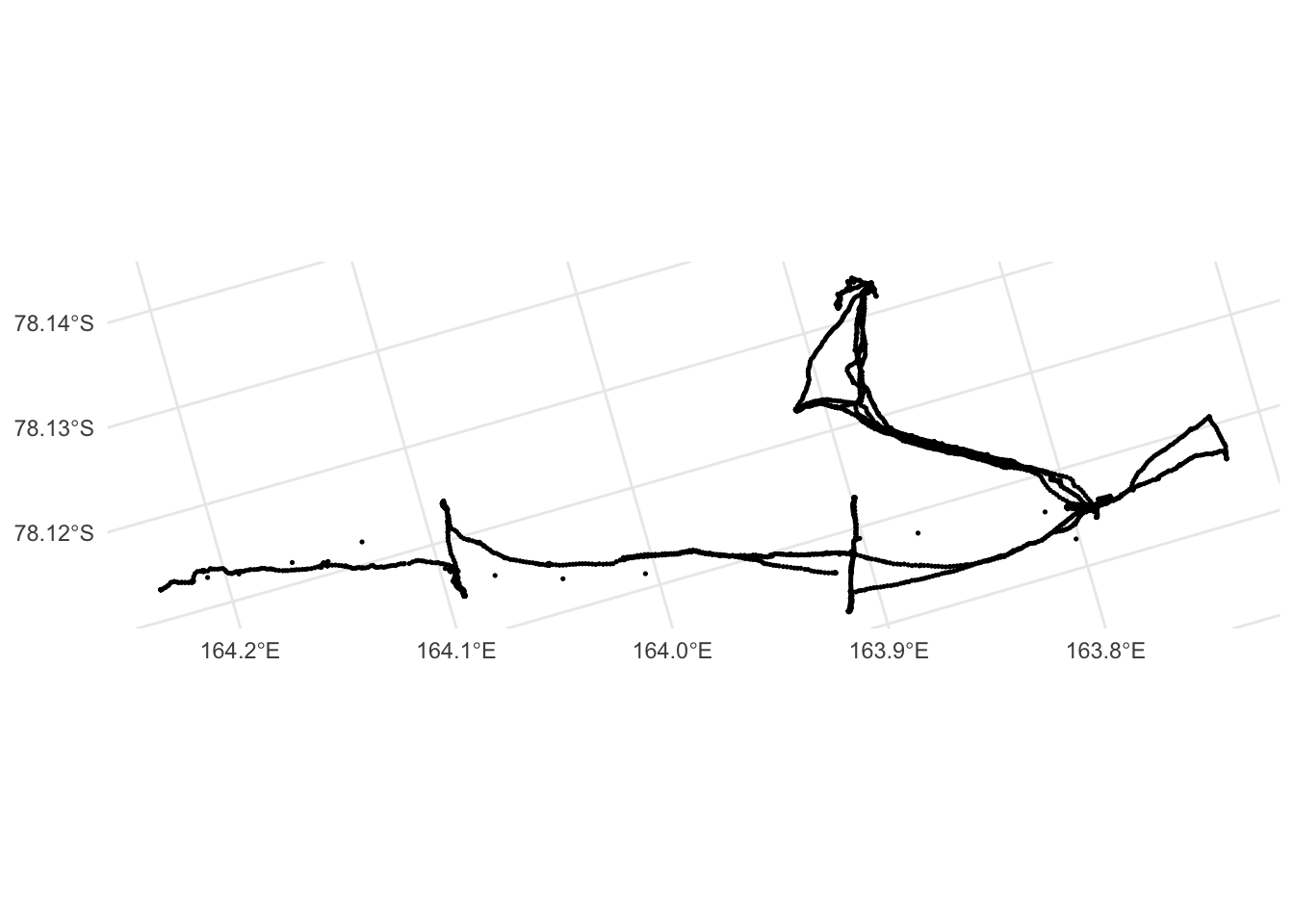
This being the case it seems reasonable to remove observations with clearly unreasonable speed estimates, assuming that these result from use of other forms of transport. However, before doing so, we augment the data with additional estimates of speed, distance, turn angle, etc. calculated from consecutive fixes (it is not advisable to remove any fixes before making these estimates).
Sanity checking the GPS estimates of speed, distance, and height
Before applying that potentially simplistic cleaning of the data, it is also reasonable to sanity check the speed, distance, and height estimates in the GPS data. First we obtain height data from a 10m DEM.
xy <- gps_data |>
  st_coordinates() |>
  as_tibble()

dem <- rast(str_glue("{here()}/_data/dem/10m/dem-10m-gps-extent.tif"))

heights_from_dem <- dem |>
  terra::extract(xy, method = "bilinear") |>
  dplyr::select(2)

TRI_from_dem <- dem |>
  terra::terrain("TRI") |>
  terra::extract(xy, method = "bilinear") |>
  select(2)

slope_from_dem <- dem |>
  terra::terrain("slope") |>
  terra::extract(xy, method = "bilinear") |>
  select(2)

xy <- xy |>
  bind_cols(heights_from_dem) |>
  bind_cols(TRI_from_dem) |>
  bind_cols(slope_from_dem) |>
  rename(Z = `dem-10m-gps-extent`,
         dem_TRI = TRI,
         dem_slope = slope)

gps_data_plus <- gps_data |>
  bind_cols(xy)
Now calculate estimates of distance, change in elevation, and slope between observations, from these numbers and from the GPS data.
gps_data_plus <- gps_data_plus |>
  mutate(
    dx1 = as.numeric(diff(as.zoo(X), na.pad = TRUE)),
    dy1 = as.numeric(diff(as.zoo(Y), na.pad = TRUE)),
    dx2 = as.numeric(diff(as.zoo(X), lag = -1, na.pad = TRUE)),
    dy2 = as.numeric(diff(as.zoo(Y), lag = -1, na.pad = TRUE)),
    dist_xy = sqrt(dx1^ 2 + dy1 ^ 2), # not useful - path followed is not straight
    turn_angle = get_turn_angle(dx1, dy1, dx2, dy2),
    dt = as.numeric(diff(as.zoo(date_time), na.pad = TRUE)),
    dh = as.numeric(diff(as.zoo(height_m), na.pad = TRUE)),
    dz = as.numeric(diff(as.zoo(Z), na.pad = TRUE))) |>
rename(
  z_gps = height_m,
  z_dem = Z)
Now some comparisons.
Distance estimates
The distance_m estimates in the provided data are generally higher than the manually calculated point to point straight line distances between fixes, which is unsurprising. However, examination of sequences of data show the two time series are well aligned (below). Differences may be due to filtering applied by the GPS unit, although this is not well documented.
gps_data_plus |>
  filter(dt == 30) |>
  slice(2:151) |>
  pivot_longer(cols = c(distance_m, dist_xy)) |>
  ggplot() +
  geom_line(aes(x = date_time, y = value, colour = name, group = name)) +
  scale_colour_manual(values = c("red", "blue"), labels = c("From XY data", "GPS estimate"), name = "Source") +
  xlab("Date/time") + ylab("Estimated distance")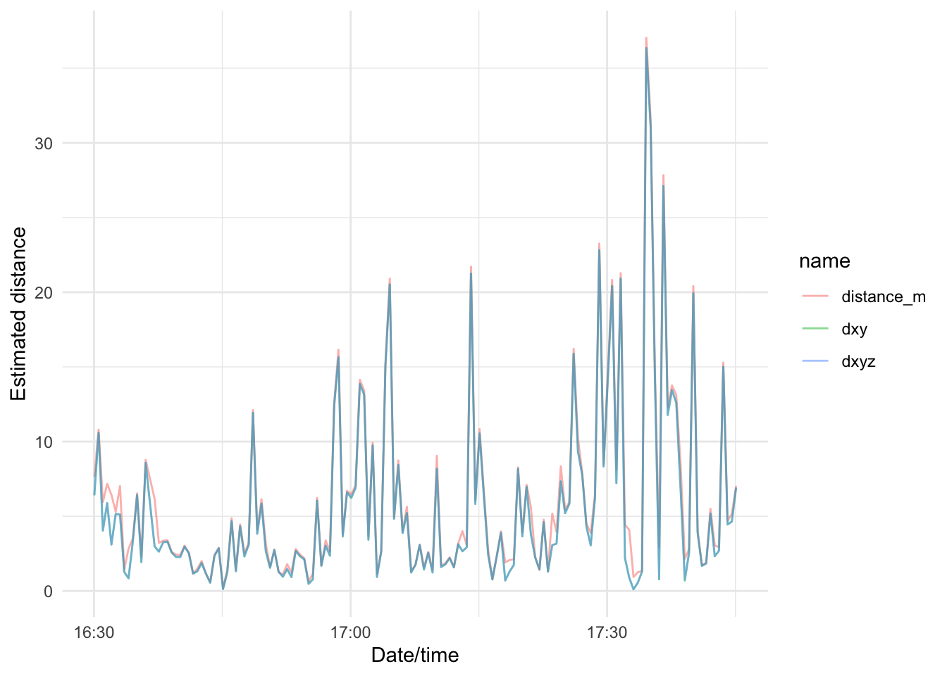
In any case, the GPS distance_m variable seems safe for use in further analysis.
Therefore we’ll remove the dist_xy alternative and rename distance_m simply to distance.
gps_data_plus <- gps_data_plus |>
  select(-dist_xy, -dx1, -dx2, -dy1, -dy2, -X, -Y) |>
  rename(distance = distance_m)
Speed estimates
Given the distance attribute we can estimate speeds for comparison with the GPS reported speed_km_h value.
gps_data_plus <- gps_data_plus |>
  mutate(derived_speed = distance / dt / 1000 * 3600)
A comparison
gps_data_plus |>
  filter(dt == 30) |>
  slice(2:151) |>
  pivot_longer(cols = c(speed_km_h, derived_speed)) |>
  ggplot() +
  geom_line(aes(x = date_time, y = value, colour = name, group = name)) +
  scale_colour_manual(values = c("red", "blue"), labels = c("Derived", "GPS estimate"), name = "Source") +
  xlab("Date/time") + ylab("Estimated speed")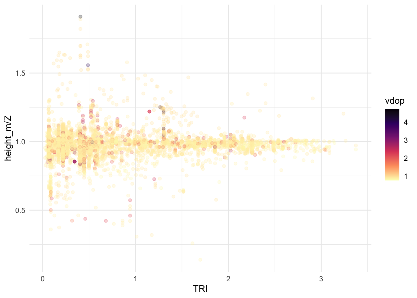
The GPS provided estimates are generally higher although there is some alignment between the time series, insofar as extended periods of lower speeds tend to line up.
The likely reason for the differences is that in a 30 second period (the usual interval between fixes) an individual may move in many directions so that the direct point to point distance between fixes is less than might be expected based on the recorded speed. So, for example, in the above chart between 16:30 and 16:40 the person was moving not in straight lines, where in the following 10 minutes they were moving in relatively straight lines. We can test this theory, at least qualitatively, by calculating a sinuosity estimate between fixes.
sinuosity <- gps_data_plus |>
  filter(dt == 30) |>
  slice(2:61) |>
  mutate(sinuosity = speed_km_h / 120 / distance,
         date_time_start = lag(date_time))

speeds <- sinuosity |>
  pivot_longer(cols = c(speed_km_h, derived_speed))

ggplot(speeds) +
  geom_step(aes(x = date_time, y = value, group = name, linetype = name),
            direction = "vh", lwd = 0.5) +
  scale_linetype_manual(values = c("dashed", "solid"), labels = c("Derived", "GPS est."), name = "Source") +
  geom_segment(data = sinuosity,
               aes(x = date_time_start, xend = date_time,
                   y = speed_km_h, colour = rank(-sinuosity)), lwd = 2) +
  scale_colour_distiller(palette = "Reds", direction = 1, name = "Rank of sinuosity") +
  xlab("Date/time") + ylab("Estimated speed")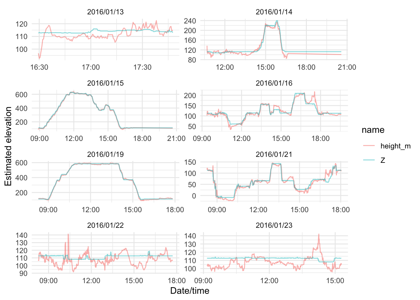
Since the estimated sinuosity here is based only on the GPS estimated speed and point to point distances, that it is generally highest (lower rank, paler reds) when the difference between the GPS reported speed speed_km_h and the manually estimated speed derived_speed is largest supports the assumption that the GPS is reporting speed using satellite carrier signal doppler effects, and not elapsed distance and time.
It therefore makes sense to use the GPS estimated speed and delete the derived speed.
gps_data_plus <- gps_data_plus |>
  select(-derived_speed) |>
  rename(speed = speed_km_h)
GPS height and elevation from the DEM
Now we consider the GPS estimated height and DEM derived elevations.
Again, there are differences between heights recorded by the GPS units, and heights extracted from the 10m DEM. It is difficult to know why these might occur, although there is a clear correlation between the two. However, there is no obvious correlation with, e.g., surface roughness (TRI), for example, or with the vertical dilution of precision (vdop) in the differences between the two:
ggplot(gps_data_plus |>
         filter(dt == 30, distance < 100, z_gps > 0, z_dem > 0) |>
         mutate(z_error = (2 * (z_gps - z_dem) / (z_gps + z_dem)))) +
  geom_point(aes(x = dem_TRI, y = z_error, colour = vdop), alpha = 0.5, size = 1) +
  scale_colour_viridis_c(option = "A", direction = -1)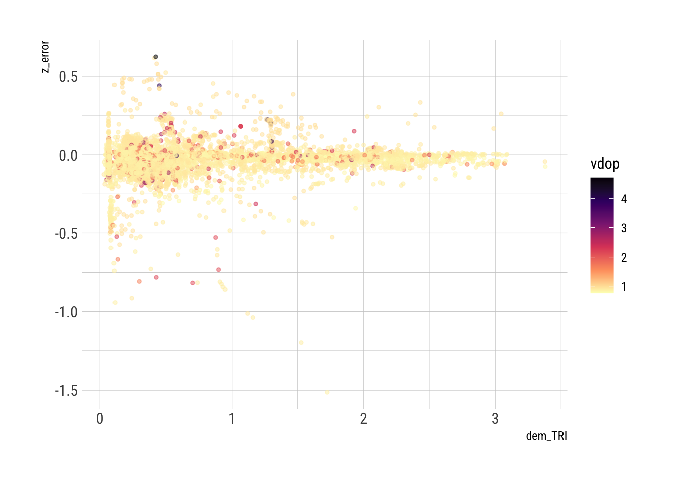
Some reassurance that the GPS height estimates are suitably aligned is obtained by plotting each days set of observations of the two as time series. On days where much of the activity occurred at the same elevation or across a very limited elevation range there are obvious deviations, but these are relatively small in magnitude; on days when more elevation chance is observed, the overall profile of the day’s activity matches well.
gps_data_plus |>
  filter(dt == 30) |>
  pivot_longer(cols = c(z_gps, z_dem)) |>
  ggplot() +
  geom_line(aes(x = date_time, y = value, colour = name, group = name), alpha = 0.5) +
  xlab("Date/time") + ylab("Estimated elevation") +
  facet_wrap(~ date, scales = "free", ncol = 2) +
  theme_minimal()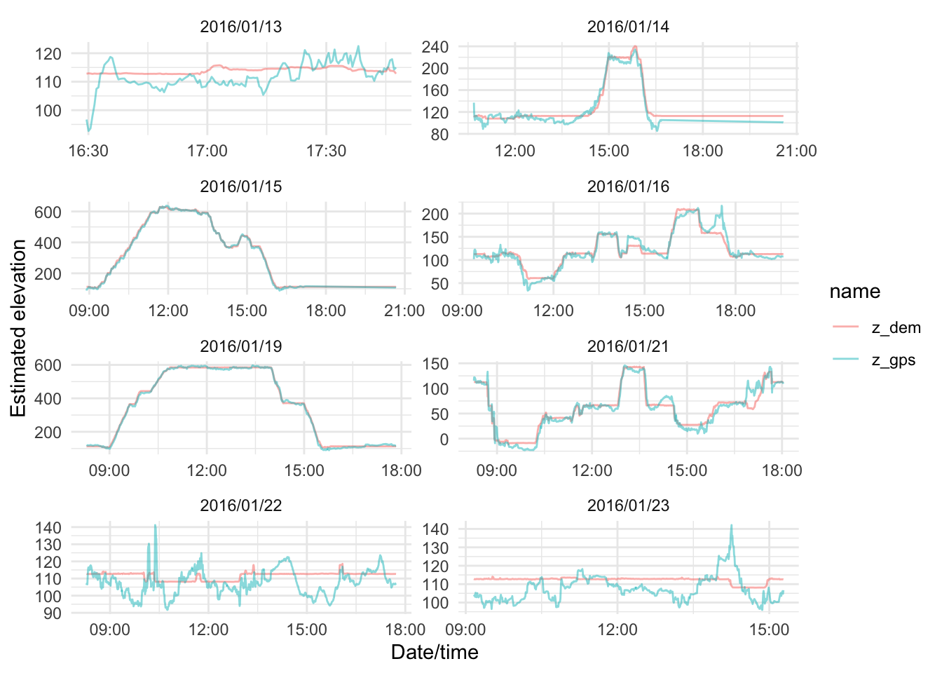
It’s not clear which is to be preferred. So add slope variables to the data:
gps_data_plus <- gps_data_plus |>
  select(-dem_TRI, -dem_slope) |>
  mutate(
    slope_gps = dh / distance,
    slope_dem = dz / distance)
We can eyeball how the choice of height measures affects the slope - speed relationship we are interested in for hiking function estimation.
df <- bind_rows(
  gps_data_plus |> mutate(slope = slope_gps, slope_src = "GPS"),
  gps_data_plus |> mutate(slope = slope_dem, slope_src = "DEM")
)

ggplot(df |> filter(dt == 30, speed < 10)) +
  geom_point(aes(x = slope, y = speed), size = 0.1, alpha = 0.5) +
  # scale_colour_viridis_c(option = "A", direction = -1) +
  # guides(colour = guide_legend(override.aes = list(size = 5))) +
  geom_smooth(aes(x = slope, y = speed)) +
  facet_wrap( ~ slope_src, labeller = "label_both") +
  theme_minimal()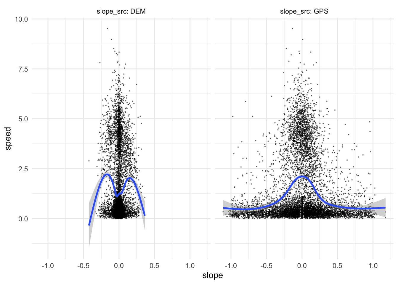
This result strongly suggests that it is a safer option to use the GPS estimates of height, although it is really not clear that it is ‘better’ or more accurate.
A hiking function
A hiking function relates slope of the land to speed at which it is traversed. Using the GPS unit reported speed and slope derived from GPS unit reported distance and height, locally estimated scatter plot smoothing yields an approximately Gaussian curve with the peak speed at or close to 0 slope. This gives some confidence that we can use these data to estimate hiking functions. The approach implied in this plot is insufficient, as the data contain many fixes that don’t give much information about ‘hiking’ as such. The preponderance of higher turn angle fixes in the less ‘mobile’ parts of the data (i.e. at lower speeds) suggests that it may be possible to filter out those data points.
Better estimation of a hiking function is left to later notebooks (see Estimating a hiking function and Refining hiking functions).
# gps_data_plus |>
#   # here's a possible filter to apply to the data to improve the estimation
#   filter(dt == 30, speed_km_h < 10, !is.na(slope_h), distance_m > 2.5, turn_angle < 150) |>
#   ggplot(aes(x = slope_h, y = speed_km_h, colour = turn_angle)) +
#   geom_point(size = 0.25) +
#   geom_smooth(aes(x = slope_h, y = speed_km_h))
#
# model <- loess(speed_km_h ~ slope_h, data = gps_data_plus)

gps_data_plus |>
  # here's a possible filter to apply to the data to improve the estimation
  filter(dt == 30, speed < 10, !is.na(slope_gps), distance > 2.5, turn_angle < 150) |>
  ggplot(aes(x = slope_gps, y = speed, colour = turn_angle)) +
  geom_point(size = 0.25) +
  geom_smooth(aes(x = slope_gps, y = speed))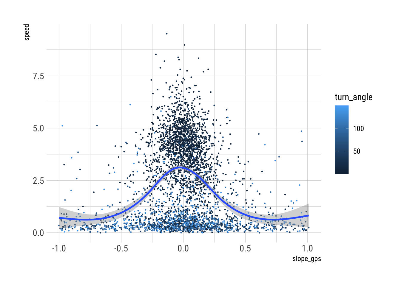
model <- loess(speed ~ slope_gps, data = gps_data_plus)Many data in the above plot are probably from ‘milling about’ in breaks, at camp, or around experiments, rather than while on the move. The best way to remove these sections is probably based on turn angles.
Conclusion: a reasonable GPS file cleaning function
Based on this exploration, GPS data need to be processed as follows (note that no initial conversion to a spatial format is required at this stage, since none of the added spatial data introduced above is required).
- Read raw data from CSV.
- Clean names with
janitor::clean_names. - Remove meaningless variable
x. - Add a
namereflecting the id of the person whose data is. - Augment data with
dt(time interval between fixes),dh(height change between fixes),slope_h(estimated slope between fixes), andturn_angle(change in direction at this fix). - Remove data outside expected latitudinal range (> -78 latitude).
- Remove fixes with high estimated speeds (>~ 10km/h).
- Remove fixes with long estimated distances (>~ 60m).
- Identify breaks in the series where
dt != 30and tag subsets of the data accordingly. - Count number of fixes in each subset – consider removing small ones…
- Drop NAs and any rows where
dt != 30.
This is the basis for a function get_cleaned_gps_data() in the script gps-data-utils.R used for cleaning up / augmenting the raw CSV files.
Footnotes
Rees WG. 2004. Least-cost paths in mountainous terrain. Computers & Geosciences 30(3) 203–209. doi: 10.1016/j.cageo.2003.11.001.↩︎