A hiking network with better data

Homing in on the most useful graph analysis outputs

Author

David O’Sullivan

Published

August 29, 2024

Update History

Date	Changes
2024-09-26	Added an executive summary.
2024-09-03	Added tentative conclusion pointing to need to explore performance when cutoff is introduced to betweennness calculation.
2024-09-01	Cleaned up to show the workflow.
2024-08-29	Initial post.

TL;DR Executive summary

The key findings progressing the overall project are:

Vertex betweenness and edge betweenness maps where it seems clear that the most informative measure is the raw betweenness not any normalised derivative from it.
Imposing cutoff costs on the betweenness calculation is a refinement left for a later notebook, where it seems clear for both theoretical reasons (route planning is performed hour by hour in the field), and practical ones (calculation is MUCH faster) betweenness centrality with imposed cost cutoff settings are the most useful graph analytic output for this project.

The primary purpose of this notebook is to show the overall workflow for making a map of potential impacts from scientists moving around in the Dry Valleys, based on slope, landcover, and hiking function inputs. The workflow is shown with respect to the 5th largest area of contiguous rocky (rocks and/or gravels) cover — an area of about 320 sq.km, at a resolution of 100m.

Much of this code is in previous notebooks in similar form, but pointing here to different data resources, and once final inputs (primarily landcover costs and a hiking function) are determined, can be automated to run on several zones across all of the Dry Valleys.

Code

library(here)
library(stringr)
library(ggplot2)
library(ggnewscale)
library(whitebox)
library(ggpubr)
library(ggspatial)
library(scales)

source(str_glue("{here()}/scripts/raster-to-graph-functions.R"))

Set up folders and some base parameters

The set up of data subfolders under the top level _data folder is:

Folder	Contents
`dry-valleys/output`	Outputs - primarily the graph and elevation data (as points) with relative movement costs
`contiguous-geologies`	GPKG files `dry-valleys-extent-??.gpkg` with a single contiguous geology polygon per file
`dry-valleys/common-inputs`	Various input layers as needed. Primarily relative landcover costs `*-cover-costs.gpkg`
`dem/10m`	DEM datasets in `raw` and `clipped` (to the Dry Valleys and Skelton basins) and a mosaiced and clipped DEM file `dry-valleys-combined-10m-dem-clipped.tif`
`dem/32m`	DEM datasets in `raw` and `clipped` (to the Dry Valleys and Skelton basins) and a mosaiced and clipped DEM file `dry-valleys-combined-32m-dem-clipped.tif`

Additionally, the basename for all files is dry-valleys, with DEM resolution used (32m or 10m) and the nominal hiking network resolution (without the m), which is likely to be 100 included in various output files as appropriate.

dem_resolution     <- "32m" # 10m also available, but probably not critical
resolution         <- 200   # 100 is high res for rapid iterating: use 200 while testing
impassable_cost    <- -999  # in the cover-costs file. hat-tip to ESRI

data_folder        <- str_glue("{here()}/_data")
base_folder        <- str_glue("{data_folder}/dry-valleys")
input_folder       <- str_glue("{base_folder}/common-inputs")
output_folder      <- str_glue("{base_folder}/output")
dem_folder         <- str_glue("{data_folder}/dem/{dem_resolution}")

basename           <- str_glue("dry-valleys")
dem_file           <- str_glue("{dem_folder}/{basename}-combined-{dem_resolution}-dem-clipped.tif")
landcover_file     <- str_glue("{input_folder}/{basename}-cover-costs.gpkg")

Load the terrain and crop to the extent

The extent in each case is a single area of ‘contiguous geology’ derived by dissolving all polygons in the GNS geomap data. These files are named *01.gpkg, *02.gpkg, etc., where the sequence number is from the largest to the smallest by area.

contiguous_geology <- "05"  # small one for testing
extent_file        <- str_glue("{base_folder}/contiguous-geologies/{basename}-extent-{contiguous_geology}.gpkg")
extent             <- st_read(extent_file)

terrain <- rast(dem_file) |>
  crop(extent |> as("SpatVector")) |>
  mask(extent |> as("SpatVector"))
# and for visualization
shade <- get_hillshade(terrain) |>
  as.data.frame(xy = TRUE) # this is for plotting in ggplot

It’s handy to make a couple of basemaps here

hillshade_basemap <- ggplot(shade) +
  geom_raster(data = shade, aes(x = x, y = y, fill = hillshade), alpha = 0.5) + 
  scale_fill_distiller(palette = "Greys", direction = 1) +
  guides(fill = "none") +
  annotation_scale(plot_unit = "m", height = unit(0.1, "cm")) +
  theme_void()

# this is a bit goofy, but seems to work
contours <- function(terrain) {
  stat_contour(data = terrain |> as.data.frame(xy = TRUE) |> rename(z = names(terrain)),
               aes(x = x, y = y, z = z), binwidth = 100, linewidth = 0.2, colour = "#ddaa44")
}

hillshade_basemap + 
  contours(terrain) +
  coord_equal()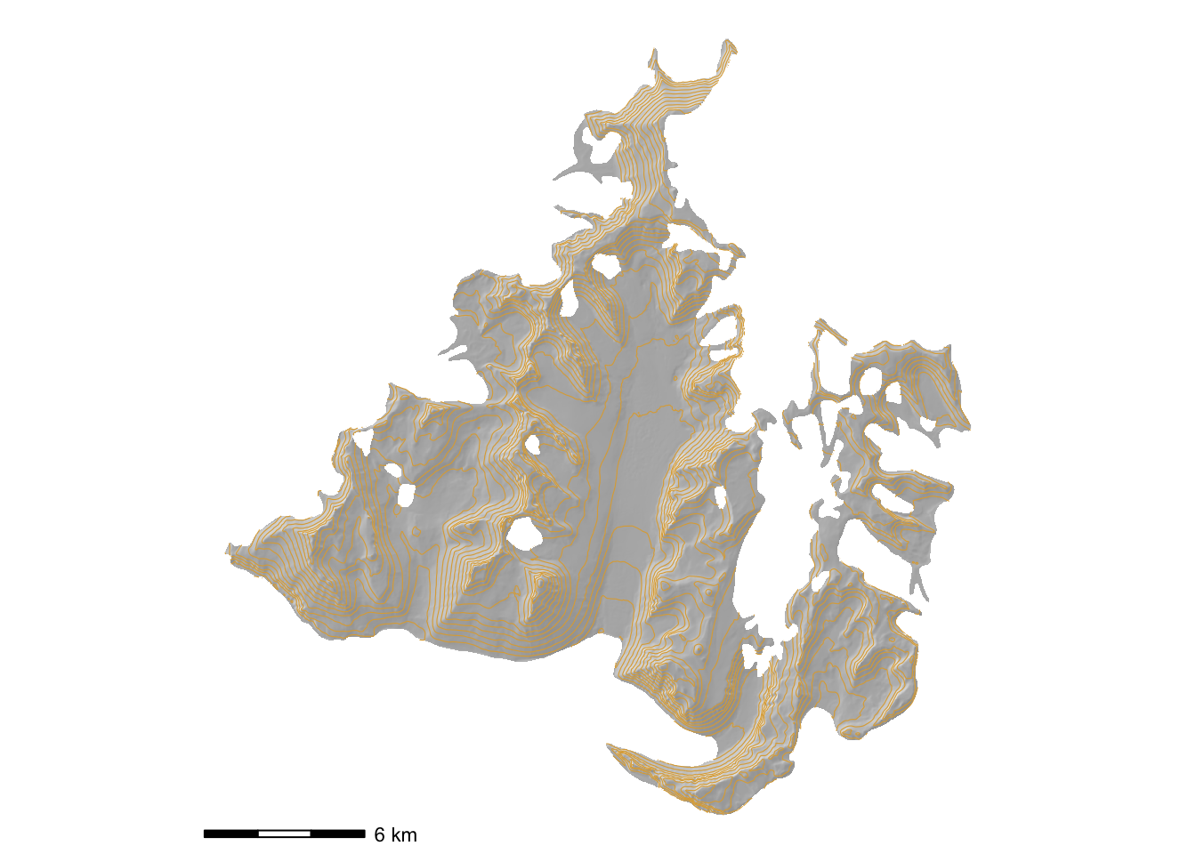

Make the graph

Nodes in the graph are centres of a hexagonal grid across the extent. The cell size of the hexagonal grid is set so that hexagons are the same area as square raster cells of side length given by resolution. The area of these is \(r^2\). The area of a hexagon with ‘radius’ \(R\) is \(3\sqrt{3}R^2/2\). Cell size in sf::st_make_grid is specified by the ‘face-to-face distance’ of the hexagons, this distance is given by \(D=\sqrt{3}R\), so \(R=D/\sqrt{3}\). Hence \[ \begin{array}{rcrcl} A & = & \frac{3\sqrt{3}}{2}\left(\frac{D}{\sqrt{3}}\right)^2 &=& r^2 \\ & & D^2 & = & \frac{2}{\sqrt{3}}r^2 \\ & & & = & r\sqrt{\frac{2}{\sqrt{3}}} \end{array} \] So make a hex grid of points with this spacing.

# calculate hexagon spacing of equivalent area
hex_cell_spacing <- resolution * sqrt(2 / sqrt(3))

# check if we have already made this dataset
hexgrid_file <- 
  str_glue("{base_folder}/output/{basename}-{contiguous_geology}-{dem_resolution}-hex-grid-{resolution}.gpkg")

if (file.exists(hexgrid_file)) {
  xy <- st_read(hexgrid_file)
} else {
  xy  <- extent |>
    st_make_grid(cellsize = hex_cell_spacing, what = "centers", square = FALSE) |>
    st_as_sf() |>
    rename(geometry = x) |>   # shouldsee https://github.com/r-spatial/sf/issues/2429
    st_set_crs(st_crs(extent))
  coords <- xy |> st_coordinates()
  xy <- xy |>
    mutate(x = coords[, 1], y = coords[, 2])
  xy |>
    st_write(str_glue(hexgrid_file), delete_dsn = TRUE)
}

Reading layer `dry-valleys-05-32m-hex-grid-200' from data source 
  `/Users/david/Documents/work/mwlr-tpm-antarctica/antarctica/_data/dry-valleys/output/dry-valleys-05-32m-hex-grid-200.gpkg' 
  using driver `GPKG'
Simple feature collection with 20777 features and 2 fields
Geometry type: POINT
Dimension:     XY
Bounding box:  xmin: 424601.4 ymin: -1262612 xmax: 452755.2 ymax: -1233391
Projected CRS: WGS 84 / Antarctic Polar Stereographic

Attach elevation values to it from the terrain data.

z <- terrain |> 
  terra::extract(xy |> as("SpatVector"), method = "bilinear")

pts <- xy |>
  mutate(z = z[, 2])

Also attach land cover relative movement costs, removing any NAs that might have been picked up along the way. These will predominantly be due to minor mismatches between the extent of the raster terrain layer and the coverage of the hexagonal grid of points. We also remove any points whose cost is equal to the sentinel value (-999) for impassable terrain (water and ice).

# remove any NAs that might result from interpolation or impassable terrain
# NAs tend to occur around the edge of study area
cover <- st_read(landcover_file)

pts <- pts |>
  st_join(cover) |>
  filter(!is.na(z), cost != impassable_cost)

Mapping it we can see that more difficult terrain is associated with the higher elevations (which are rocky).

hillshade_basemap +
  geom_sf(data = pts, aes(colour = cost), size = 0.05) +
  scale_colour_viridis_c(option = "A", direction = -1) +
  contours(terrain) +
  theme_void()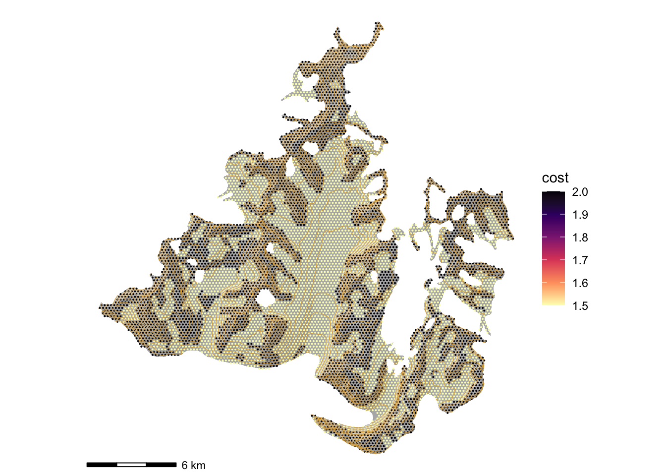

Now we make the graph by connecting pairs of points within range of one another (note 1.1 factor to catch floating-point near misses).

graph_file <-   
  str_glue("{base_folder}/output/{basename}-{contiguous_geology}-{dem_resolution}-graph-hex-{resolution}.txt") 

if (file.exists(graph_file)) {
  G <- read_graph(graph_file) 
} else {
  G <- graph_from_points(pts, hex_cell_spacing * 1.1)
  write_graph(G, graph_file)
}

# note... for now this uses a default Tobler hiking function
G <- assign_movement_variables_to_graph(G, xyz = pts, impedances = pts$cost)

Now we have a graph

So let’s take a look… first, at a map of the network for reassurance - noting that since costs are different in each direction there’s no easy way to show this unambiguously

hillshade_basemap +
  geom_sf(data = G |> get_graph_as_line_layer(), 
          aes(colour = log(cost)), linewidth = 0.05) +
  scale_colour_viridis_c(option = "A", direction = -1) +
  theme_void()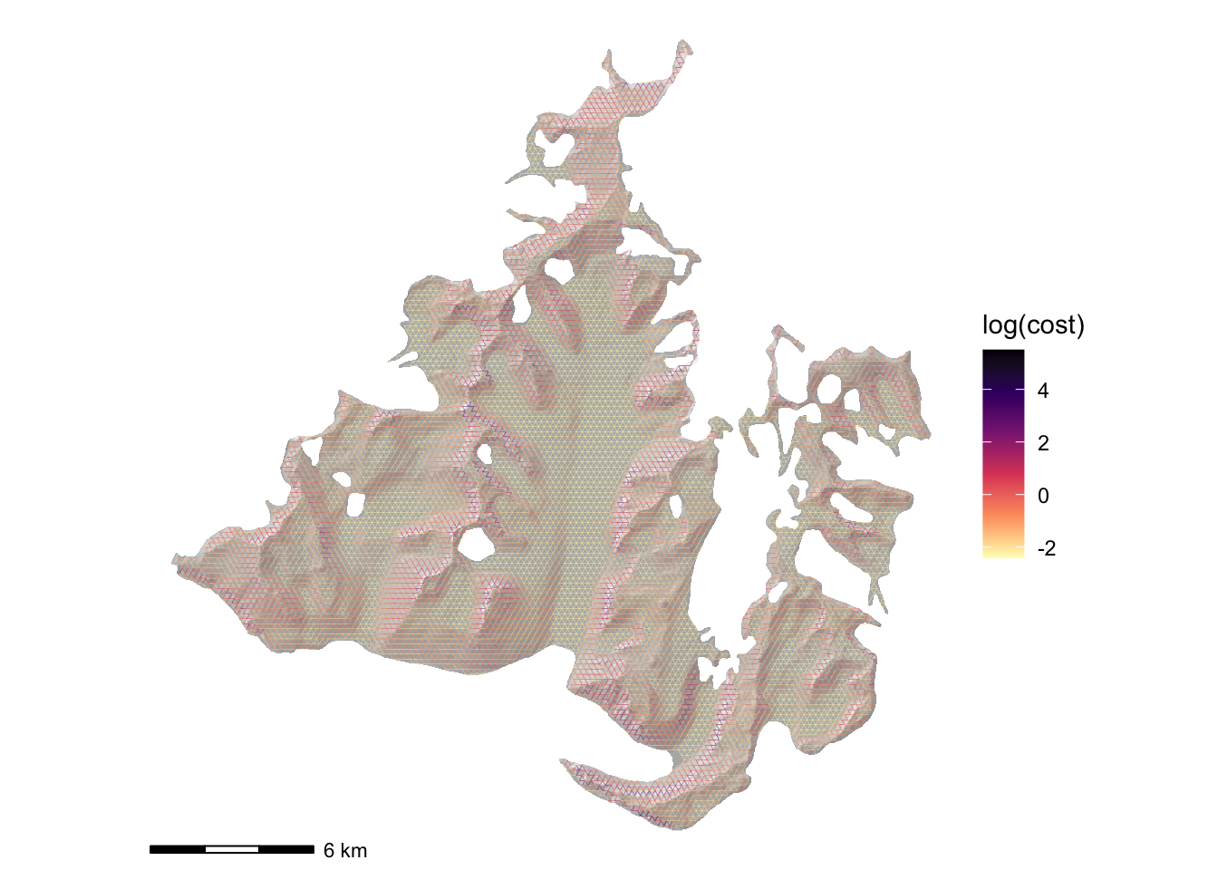

And just for assurance, here’s an estimated travel time map. These are actually tricky to make because

# pick a random point as origin point for some examples
origin_i <- sample(seq_along(pts$geom), 1)[1]
origin <- c(pts$x[origin_i], pts$y[origin_i])

V(G)$time_hrs <- distances(G, v = c(V(G)[origin_i]), 
                           weights = edge_attr(G, "cost")) |> t()
df <- vertex.attributes(G) |> as.data.frame()

hillshade_basemap +
  geom_point(data = df, aes(x = x, y = y, colour = time_hrs), size = 0.25) +
  scale_colour_viridis_c(option = "A", direction = -1) +
  annotate("point", x = origin[1], y = origin[2], pch = 4) +
  coord_equal()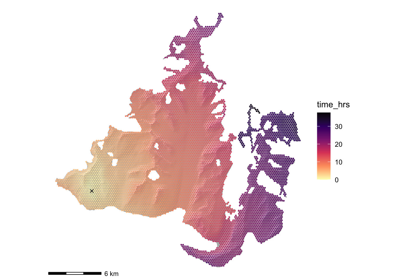

Note the following, if we want the estimated travel times as a raster layer rather than a point dataset, where we use Sibley’s natural neighbours interpolation method from whitebox_tools to interpolate to a raster from the hex grid distributed points.

[NOT RUN]

# filenames for (temporary) shapefile and TIF outputs that we need 
shp_fname <- str_glue("{here()}/_temp/test-{format(origin_i, scientific = FALSE)}-hex.shp")
tif_fname <- str_glue("{here()}/_temp/travel_time.tif")

# write the df out to a shapefile, which Whitebox Tools needs
df |> st_as_sf(coords = c("x", "y"), crs = crs(extent)) |>
  st_write(shp_fname, delete_dsn = TRUE)

# do the interpolation using Sibley's natural neighbours since we have a regular
# and relatively dense array and save it to a tif
wbt_natural_neighbour_interpolation(
  shp_fname, output = tif_fname, field = "time_hrs", base = str_glue(dem_file))

rast(tif_fname) |>
  mask(extent |> as("SpatVector")) |>
  as.data.frame(xy = TRUE) |>
  ggplot(aes(x = x, y = y)) +
  geom_raster(aes(fill = travel_time)) +
  scale_fill_viridis_c(option = "A", direction = -1, name = "Est. time hrs") +
  coord_equal() +
  annotation_scale(plot_unit = "m", height = unit(0.1, "cm")) +
  theme_void()

Shortest path tree

This is more for fun that useful – although given a set of heavily used sites (base camps?) their shortest path trees might usefully be combined to give a general idea of most at-risk / heavily travelled areas. Note that shortest_path_tree is a function in raster-graph-functions.R not an igraph built-in.

SPT <- G |>
  get_shortest_path_tree(origin_i) |>
  get_graph_as_line_layer()

ggplot() + 
  contours(terrain) +
  geom_sf(data = SPT, linewidth = 0.1) +
  geom_sf(data = pts |> slice(origin_i), pch = 4) +
  theme_void()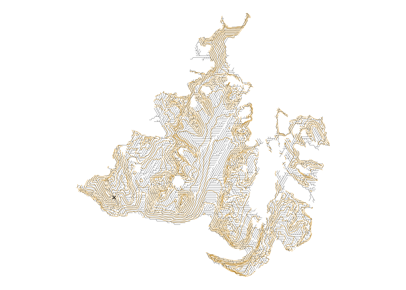

This shows all the potential most efficient pathways out from the root vertex to every other vertex. There is a strong tendency for these paths to follow contours.

Betweenness centralities

It turns out we can count all the appearances of graph edges and/or vertices in all the shortest paths among all the vertices in a network. These are graph centrality measures termed edge betweenness and vertex betweenness (the latter is often simply betweenness).

If we use these in their ‘raw’ form then the most geographically central spots in a study area may have the highest values by virtue of their location in the middle of the area. This might not be wrong — not exactly anyway — but it might lead to ignoring relatively vulnerable areas that may be heavily travelled in spite of more peripheral locations because they are at bottlenecks between parts of the study area. For this reason we calculate a base- and cost- betweenness scores. The former is the betweenness if the cost of traversing every edge in the graph was equal’ the latter is when slope and terrain are taken into account.

# vertices
# add 1 to these to make it easier to scale them if needed because a raw value 0 is possible
base_vb <- betweenness(G)
cost_vb <- betweenness(G, weights = E(G)$cost)
base_vb <- rescale(base_vb, to = c(1, 100))
cost_vb <- rescale(cost_vb, to = c(1, 100))
diff_vb <- (cost_vb - base_vb) / (cost_vb + base_vb)
rel_vb <- cost_vb / base_vb
log_rel_vb <- log(rel_vb)

# edges
base_eb <- edge_betweenness(G)
cost_eb <- edge_betweenness(G, weights = E(G)$cost)
base_eb <- rescale(base_eb, to = c(1, 100))
cost_eb <- rescale(cost_eb, to = c(1, 100))
diff_eb <- (cost_eb - base_eb) / (cost_eb + base_eb)
rel_eb <- cost_eb / base_eb
log_rel_eb <- log(rel_eb, 10)

Add all these results to the relevant graph attributes.

Gsp <- G |> 
  set_vertex_attr("base_vb", value = base_vb) |>
  set_vertex_attr("cost_vb", value = cost_vb) |>
  set_vertex_attr("diff_vb", value = diff_vb) |>
  set_vertex_attr("rel_vb", value = rel_vb) |>
  set_vertex_attr("log_rel_vb", value = log_rel_vb)|> 
  set_edge_attr("base_eb", value = base_eb) |>
  set_edge_attr("cost_eb", value = cost_eb) |>
  set_edge_attr("diff_eb", value = diff_eb) |>
  set_edge_attr("rel_eb", value = rel_eb) |>
  set_edge_attr("log_rel_eb", value = log_rel_eb)

Maps of betweenness centrality

First vertex centrality, where it is relatively simple to colour vertices by their centrality. It is useful to map all the various calculated betweenness measures to get a feel for which may be most useful.

m1 <- hillshade_basemap +
  geom_sf(data = Gsp |> get_graph_as_point_layer(),
          aes(colour = base_vb), size = 0.02) +
  scale_colour_viridis_c(option = "A", direction = -1)

m2 <- hillshade_basemap +
  geom_sf(data = Gsp |> get_graph_as_point_layer(),
          aes(colour = cost_vb), size = 0.02) +
  scale_colour_viridis_c(option = "A", direction = -1)

m3 <- hillshade_basemap +
  geom_sf(data = Gsp |> get_graph_as_point_layer(),
          aes(colour = diff_vb), size = 0.02) +
  scale_colour_distiller(palette = "RdBu") 

m4 <- hillshade_basemap +
  geom_sf(data = Gsp |> get_graph_as_point_layer(),
          aes(colour = rel_vb), size = 0.02) +
  scale_colour_viridis_c(option = "A", direction = -1)

m5 <- hillshade_basemap +
  geom_sf(data = Gsp |> get_graph_as_point_layer(),
          aes(colour = log_rel_vb), size = 0.02) +
  scale_colour_viridis_c(option = "A", direction = -1)
  
ggarrange(plotlist = list(m1, m2, m3, m4, m5), ncol = 2, nrow = 3)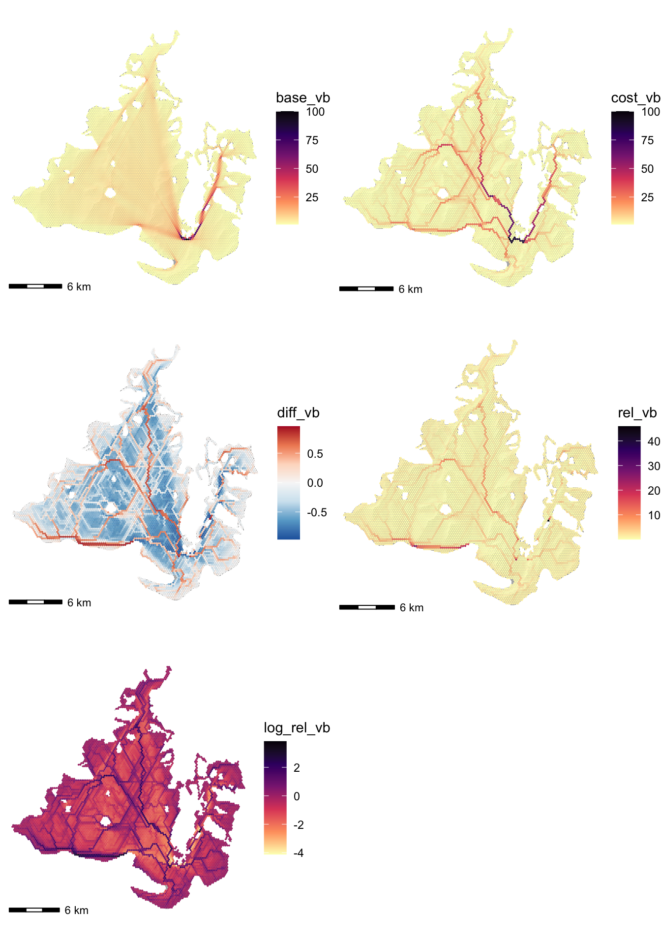

Examining these results, it appears that the the simple cost_vb betweenness may actually be the most useful in revealing routes likely to be well trafficked. The diff_vb output also appears likely to be useful.

Edge centrality is trickier to map (because of how the linewidth aesthetic works).

m1 <- hillshade_basemap +
  geom_sf(data = Gsp |> get_graph_as_line_layer() |>
            mutate(lwd = base_eb / max(E(Gsp)$base_eb)),
          aes(colour = base_eb, linewidth = lwd)) +
  scale_colour_viridis_c(option = "A", direction = -1) +
  scale_linewidth_identity()

m2 <- hillshade_basemap +
  geom_sf(data = Gsp |> get_graph_as_line_layer() |>
            mutate(lwd = cost_eb / max(E(Gsp)$cost_eb)),
          aes(colour = cost_eb, linewidth = lwd)) +
  scale_colour_viridis_c(option = "A", direction = -1) +
  scale_linewidth_identity()

m3 <- hillshade_basemap +
  geom_sf(data = Gsp |> get_graph_as_line_layer(),
          aes(colour = diff_eb), linewidth = 0.1) +
  scale_colour_distiller(palette = "RdBu") 

m4 <- hillshade_basemap +
  geom_sf(data = Gsp |> get_graph_as_line_layer(),
          aes(colour = rel_eb), linewidth = 0.1) +
  scale_colour_distiller(palette = "RdBu") 

m5 <- hillshade_basemap +
  geom_sf(data = Gsp |> get_graph_as_line_layer(),
          aes(colour = log_rel_eb), linewidth = 0.1) +
  scale_colour_distiller(palette = "RdBu") 
  
ggarrange(plotlist = list(m1, m2, m3, m4, m5), ncol = 2, nrow = 3)

Here, it seems clear that the cost_eb is likely to be the most useful output.

Conclusions

Tentatively, I conclude from the above that the most useful outputs are the vertex cost-based betweenness and difference outputs. The edge betweenness results are similar, harder to map, and double the computation times without adding much.

The next step is to investigate the impact on computation times of imposing a ‘cutoff’ time on vertex betweenness measures. Some initial exploration suggests that this greatly speeds up computation, again, without necessarily leading to very different conclusions concerning likely areas of high impact.