Building a hiking network

Also a work in progress…

Update History

Date	Changes
2024-09-26	Added an executive summary.
2024-08-06	Initial post.

TL;DR Executive summary

The key findings are:

• Essential steps in building a hiking network are set out and remain valid.
• The interpolation step in Making an estimated travel time map is overkill: it is sufficient for mapping purposes to display a point map of the graph vertices.
• An additional necessary step became apparent in later work where very steep edges remain in the networks. These may not matter much in practice as shortest path network approaches are unlikely to highlight them as plausible routes (some very steep edges end up with multi-hour traversal time estimates!). However, it makes sense to remove such edges completely from consideration, and if that makes some regions completely inaccessible this is probably a more realistic outcome.

  ---

This notebook explores creation of hiking networks across a terrain where movement rates may depend on the direction of movement (because going uphill is different than going downhill…).

First we set up some folders and filenames.

library(here)
library(stringr)
library(ggplot2)
library(ggnewscale)
library(whitebox)

source(str_glue("{here()}/scripts/raster-to-graph-functions.R"))

base_folder <-    str_glue("{here()}/_data/testing")
input_folder <-   str_glue("{base_folder}/input")
output_folder <-  str_glue("{base_folder}/output")
basename <-       "dry-valleys-10m"
dem_file <-       str_glue("{input_folder}/{basename}.tif")
imagery_file <-   str_glue("{input_folder}/{basename}-imagery.tif")
landcover_file <- str_glue("{input_folder}/{basename}-cover-costs.gpkg")
extent_file <-    str_glue("{input_folder}/{basename}-extent.gpkg")
origins_file <-   str_glue("{input_folder}/{basename}-origins.gpkg")

Now read in the DEM and an extent, and imagery (which we might not use…).

terrain <- rast(dem_file)
# and for visualization
shade <- get_hillshade(terrain)
imagery <- rast(imagery_file)
extent <- st_read(extent_file)

# make a focal area for convenience of plotting in some situations
centre_of_extent <- extent |> 
  st_centroid() # we use this later...
c_vec <- centre_of_extent |>
  st_coordinates() |>
  as.vector()
focal_area <- ((extent$geom[1] - c_vec) * diag(0.025, 2, 2) + c_vec) |>
  st_sfc(crs = st_crs(extent)) |>
  st_as_sf() |>
  rename(geom = x)

Setup a resolution for use in building networks (i.e. determining which cells are adjacent to one another in vector GIS space). Although we have a DEM at 10m resolution, at least for now we’ll use a coarser grain for construction of the network. It is in any case unclear what an appropriate resolution might be given the various approximations in play.

# assume square pixels: 50m on a side
resolution <- res(terrain)[1] * 5 
# calculate hexagon spacing of equivalent area
hex_cell_spacing <- 2 * resolution / sqrt(2 * sqrt(3))

hexgrid_file <- str_glue("{input_folder}/{basename}-hex-grid-{resolution}.gpkg")
graph_file <-   str_glue("{output_folder}/{basename}-graph-hex-{resolution}.txt") 

hex_resolution is a hexagon spacing for use in st_make_grid that yields the same area cell as square cells with edge length given by resolution

Making a hex grid across the terrain

We build the network based on hex spaced points, not a square grid. This is helpful in making all edges the same length, as opposed to in a square grid where diagonal neighbour cell centres are further apart than edge neighbouring cells.

We load a hex grid file if one has already been made, otherwise build it.

IMPORTANT NOTE: Don’t forget to remake this grid if changing any of the code prior to this point in the workflow in ways that affect the spacing of the hex grid.

if (file.exists(hexgrid_file)) {
  xy <- st_read(hexgrid_file)
} else {
  xy  <- extent |>
    st_make_grid(cellsize = hex_cell_spacing, what = "centers", square = FALSE) |>
    st_as_sf() |>
    st_set_crs(st_crs(extent))
  xy |>
    st_write(str_glue(hexgrid_file), delete_dsn = TRUE)
}

Make a plot to make sure things are the right scale, in particular that the hexes we get are the same area as the simple square grid cells would be (this isn’t critical, but it’s nice as a standardisation of what ‘resolution’ means for a hex grid).

square_grid <- focal_area |>
  st_make_grid(cellsize = resolution)

ggplot(square_grid) +
  geom_sf(colour = "white") +
  geom_sf(data = xy |> st_filter(focal_area), colour = "red", size = 3) +
  theme_void()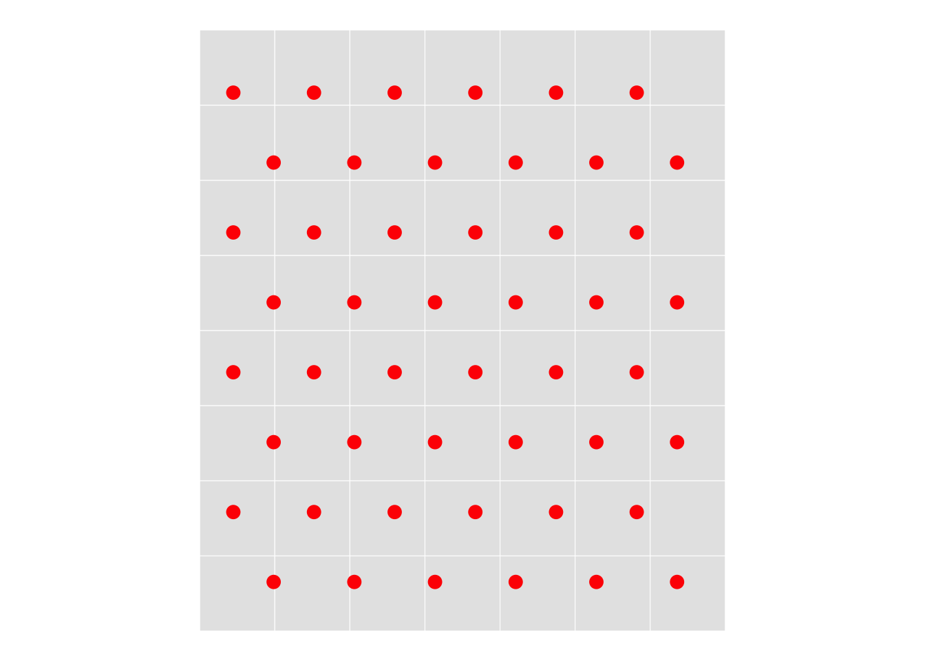

By visual inspection these are similar. We can confirm that the hexagon area in a grid at this spacing is

focal_area |> 
  st_make_grid(cellsize = hex_cell_spacing, square = FALSE) |> 
  head(1) |> 
  st_area()

2500 [m^2]

which is the same as the square grid

square_grid |> head(1) |> st_area()

2500 [m^2]

Retrieve elevations from the terrain

Although we do the modelling of hiking functions using elevations in the GPS data, we don’t have complete elevation data for the area on that basis, so we retrieve these from the DEM.

z <- terrain |> 
  terra::extract(xy |> as("SpatVector"), method = "bilinear")
# make pts and remove any NAs that might result from interpolation
# NAs are around the edges of the study area
pts <- xy |>
  mutate(z = z[, 2]) |>
  filter(!is.na(z))

Again a map is helpful, although again we use only the focal area so we can see what’s going on—and for speed of plotting.

ggplot(pts |> st_filter(focal_area)) +
  geom_sf(aes(colour = z), size = 20) +
  scale_colour_distiller(palette = "Oranges") +
  theme_void()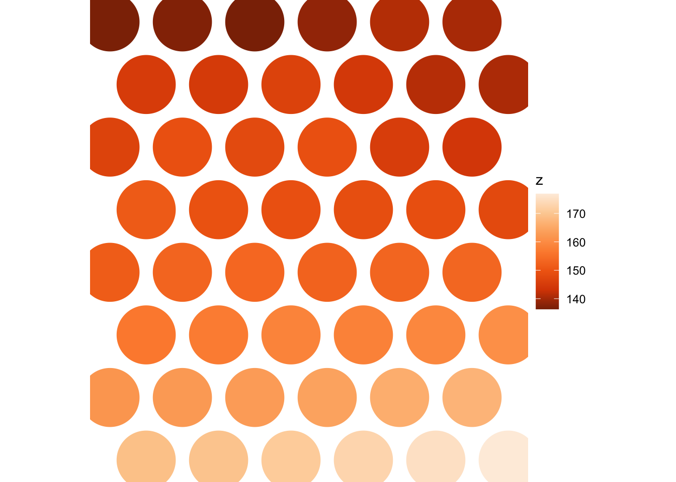

Make a graph (i.e. network) connecting these elevation points

The graph_from_points function in raster-to-graph-functions.R creates an igraph::graph object from an (x, y) point set. IMPORTANT NOTE: Don’t forget to remake the graph if messing with any of the code above here that might affect the spacing of the hex grid.

if (file.exists(graph_file)) {
  G <- read_graph(graph_file) 
} else {
  G <- graph_from_points(pts, hex_cell_spacing * 1.1)
  write_graph(G, graph_file)
}

Before we can visualize this easily, we have to attach various data to its elements (at the moment it is just a set of vertices without any attributes). The required data include a landcover layer with relative impedances. Note that for now this cover layer is entirely made up – pending consultation with someone more knowledgeable about conditions on the ground. As far as I can tell from imagery the high cost areas are ‘ice’ which I’ve arbitrarily assigned a relative cost of 5.

cover <- st_read(landcover_file)

ggplot() +
  geom_sf(data = cover, aes(fill = as.factor(cost)), linewidth = 0) +
  scale_fill_manual(values = c("white", "red"), name = "Relative cost") +
  # some ggnewscale shenanigans required to plot a second layer with fill aesthetic
  new_scale_fill() +
  geom_raster(data = shade |> as.data.frame(xy = TRUE), 
              aes(x = x, y = y, fill = hillshade), alpha = 0.5) + 
  scale_fill_distiller(palette = "Greys", direction = 1) +
  guides(fill = "none") +
  theme_void()

Next add attributes to the graph using the assignment_movement_variables_to_graph function in raster-to-graph-functions.R

xyz <- extract_xyz_from_points(pts)

costs <- pts |>
  st_join(cover, .predicate = st_within) |>
  st_drop_geometry() |>
  select(cost)

# note... for now this uses a default Tobler hiking function
G <- assign_movement_variables_to_graph(G, xyz, impedances = costs$cost)

Now we have a graph with coordinates assigned to its vertices, we can map it (after transforming to a sf dataset)

ggplot(G |> get_graph_as_line_layer() |> 
  st_filter(focal_area)) +
  geom_sf(aes(colour = cost)) +
  theme_void()

It’s not clear above that this is a bidirectional network, but we can see by inspection, e.g. the first edge in the graph is between vertices 1 and 166. We can access these (in igraph’s rather abstruse way), as follows:

G |> 
  edge_attr(index = get.edge.ids(G, c(1, 166, 166, 1))) |>
  as_tibble()

length_xyz	length_xy	z_diff	gradient	impedance	tobler_speed	cost
53.72997	53.7285	-0.3975143	-0.0073986	1	3101.323	0.0173249
53.72997	53.7285	0.3975143	0.0073986	1	2944.794	0.0182457

The lengths of the edges are identical, their height differences and gradients are opposite and the speed (metres per hour) and cost (time to traverse in hours) are different due to the slope.

Make an estimated travel time map

Using the graph representation we can estimate travel times from any start location to every other location. For the sake of illustration we’ll make such a map from the graph vertex closest to the centre of the study area.

origin_i <- centre_of_extent |>
  st_nearest_feature(pts)

V(G)$time_hrs <- distances(G, v = c(V(G)[origin_i]), weights = edge_attr(G, "cost")) |> t()

# assemble results into a DF
df <- data.frame(x = V(G)$x, y = V(G)$y, z = V(G)$z, 
                 time_hrs = V(G)$time_hrs, 
                 cost = costs$cost)
# write this out to a shapefile, which Whitebox Tools needs
shp_fname <- str_glue("{here()}/_temp/{basename}-{format(origin_i, scientific = FALSE)}-hex.shp")
df |> st_as_sf(coords = c("x", "y"), crs = crs(extent)) |>
  st_write(shp_fname, delete_dsn = TRUE)

# note that interpolation is required because we are using hexagonal grid cells
# do interpolation using Sibley's natural neighbours since we have a regular
# and relatively dense array and save it to a tif
tif_fname <- str_glue("{here()}/_temp/travel_time.tif")
wbt_natural_neighbour_interpolation(shp_fname, field = "time_hrs",
                                    output = tif_fname, 
                                    base = str_glue(dem_file))

Reading the exported raster layer made by whitebox::wbt_natural_neighbour_interpolation back in we get a map of estimated travel times.

rast(tif_fname) |>
  as.data.frame(xy = TRUE) |>
  ggplot(aes(x = x, y = y)) +
  geom_raster(aes(fill = travel_time)) +
  scale_fill_distiller(palette = "Spectral", name = "Est. time hrs") +
  geom_contour(aes(z = travel_time), linewidth = 0.5) +
  coord_equal() +
  theme_void()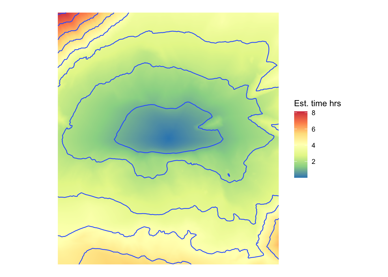

In practice we’ll use other graph functionalities than one origin to all destination shortest paths, but this gives the general idea.