Exploring hiking network options

Also a work in progress…

Author

David O’Sullivan

Published

August 7, 2024

Update History

Date	Changes
2024-09-26	Added an executive summary.
2024-08-07	Initial post.

TL;DR Executive summary

The key findings are:

Estimated travel time maps are easily produced, but only show travel time from a single origin. This might have use for a base camp location, but otherwise seems to have limited value.
Some graph derivatives are interesting but unlikely to be especially useful, e.g. shortest path tree, minimum spanning tree.
The most promising approach is centrality measures on the graph. Among the options available the most promising class of measures are betweennees measures since these focus attention on graph edges and vertices most often traversed along the shortest routes among vertices.
Both vertex and edge betweenness are available options. Only the latter is explored here, but vertex betweenness is more readily visualized and in later notebooks the two approaches lead to essentially the same conclusions.

Per the previous notebook we’ll make a small network (lower resolution) so we can explore the possibilities of this graph representation.

Code

library(here)
library(stringr)
library(ggplot2)
library(ggnewscale)
library(whitebox)
library(ggpubr)

source(str_glue("{here()}/scripts/raster-to-graph-functions.R"))

base_folder <-    str_glue("{here()}/_data/testing")
input_folder <-   str_glue("{base_folder}/input")
output_folder <-  str_glue("{base_folder}/output")
basename <-       "dry-valleys-10m"
dem_file <-       str_glue("{input_folder}/{basename}.tif")
imagery_file <-   str_glue("{input_folder}/{basename}-imagery.tif")
landcover_file <- str_glue("{input_folder}/{basename}-cover-costs.gpkg")
extent_file <-    str_glue("{input_folder}/{basename}-extent.gpkg")
origins_file <-   str_glue("{input_folder}/{basename}-origins.gpkg")

terrain <- rast(dem_file)
# and for visualization
shade <- get_hillshade(terrain)
imagery <- rast(imagery_file)
extent <- st_read(extent_file)

# make a focal area for convenience of plotting in some situations
centre_of_extent <- extent |> 
  st_centroid() # we use this later...
c_vec <- centre_of_extent |>
  st_coordinates() |>
  as.vector()
focal_area <- ((extent$geom[1] - c_vec) * diag(0.025, 2, 2) + c_vec) |>
  st_sfc(crs = st_crs(extent)) |>
  st_as_sf() |>
  rename(geom = x)

resolution <- res(terrain)[1] * 20 
# calculate hexagon spacing of equivalent area
hex_cell_spacing <- 2 * resolution / sqrt(2 * sqrt(3))

hexgrid_file <- str_glue("{input_folder}/{basename}-hex-grid-{resolution}.gpkg")
graph_file <-   str_glue("{output_folder}/{basename}-graph-hex-{resolution}.txt") 

if (file.exists(hexgrid_file)) {
  xy <- st_read(hexgrid_file)
} else {
  xy  <- extent |>
    st_make_grid(cellsize = hex_cell_spacing, what = "centers", square = FALSE) |>
    st_as_sf() |>
    st_set_crs(st_crs(extent))
  xy |>
    st_write(str_glue(hexgrid_file), delete_dsn = TRUE)
}

z <- terrain |> 
  terra::extract(xy |> as("SpatVector"), method = "bilinear")
# make pts and remove any NAs that might result from interpolation
# NAs are around the edges of the study area
pts <- xy |>
  mutate(z = z[, 2]) |>
  filter(!is.na(z))

if (file.exists(graph_file)) {
  G <- read_graph(graph_file) 
} else {
  G <- graph_from_points(pts, hex_cell_spacing * 1.1)
  write_graph(G, graph_file)
}

cover <- st_read(landcover_file)

xyz <- extract_xyz_from_points(pts)

costs <- pts |>
  st_join(cover, .predicate = st_within) |>
  st_drop_geometry() |>
  select(cost)

# note... for now this uses a default Tobler hiking function
G <- assign_movement_variables_to_graph(G, xyz, impedances = costs$cost)

Now we have a graph

So let’s take a look…

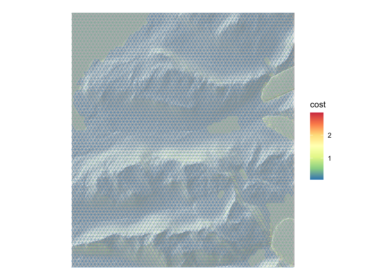
# make a hillshade 'basemap'
hillshade_basemap <- ggplot() +
  geom_raster(data = shade |> as.data.frame(xy = TRUE), 
              aes(x = x, y = y, fill = hillshade), alpha = 0.5) + 
  scale_fill_distiller(palette = "Greys", direction = 1) +
  guides(fill = "none") +
  theme_void()

hillshade_basemap +
  geom_sf(data = G |> get_graph_as_line_layer(), 
          aes(colour = cost), linewidth = 0.1) +
  scale_colour_distiller(palette = "Spectral") +
  theme_void()

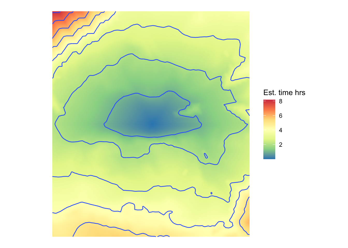
And just for assurance, here’s the estimated travel time map.

origin_i <- centre_of_extent |>
  st_nearest_feature(pts)

V(G)$time_hrs <- distances(G, v = c(V(G)[origin_i]), weights = edge_attr(G, "cost")) |> t()

# assemble results into a DF
df <- data.frame(x = V(G)$x, y = V(G)$y, z = V(G)$z, 
                 time_hrs = V(G)$time_hrs, 
                 cost = costs$cost)
# write this out to a shapefile, which Whitebox Tools needs
shp_fname <- str_glue("{here()}/_temp/{basename}-{format(origin_i, scientific = FALSE)}-hex.shp")
df |> st_as_sf(coords = c("x", "y"), crs = crs(extent)) |>
  st_write(shp_fname, delete_dsn = TRUE)

# do the interpolation using Sibley's natural neighbours since we have a regular
# and relatively dense array and save it to a tif
tif_fname <- str_glue("{here()}/_temp/travel_time.tif")
wbt_natural_neighbour_interpolation(shp_fname, field = "time_hrs",
                                    output = tif_fname, 
                                    base = str_glue(dem_file))

Reading the exported raster layer made by whitebox::wbt_natural_neighbour_interpolation back in we get a map of estimated travel times.

rast(tif_fname) |>
  as.data.frame(xy = TRUE) |>
  ggplot(aes(x = x, y = y)) +
  geom_raster(aes(fill = travel_time)) +
  scale_fill_distiller(palette = "Spectral", name = "Est. time hrs") +
  geom_contour(aes(z = travel_time), linewidth = 0.5) +
  coord_equal() +
  theme_void()

It may be worth noting that this map made with a 200m resolution network doesn’t differ greatly from the one at 50m resolution in the previous notebook.

OK… so what can we do with these things?!

The network is stored as an igraph object G. This admits many different network analysis methods.

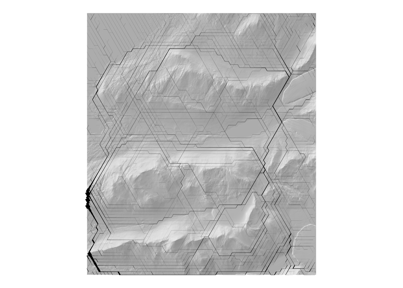
Minimum spanning tree

This is the shortest total path length (expressed here in the estimated traversal time variable cost) to reach all graph nodes.

MST <- G |> 
  mst(weights = E(G)$cost) |>
  get_graph_as_line_layer()

We can see what this looks like

hillshade_basemap + 
  geom_sf(data = MST, linewidth = 0.1)

The hillshade basemap highlights how the total shortest path prioritises paths that follow contours since the lowest cost way in general to get to a particular vertex is from a neighbouring vertex at similar elevation.

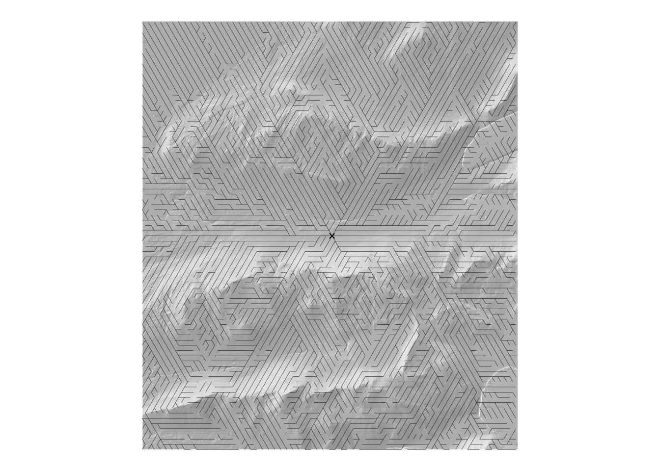
Shortest path tree

Starting from a given vertex we can make a tree graph which shows all the shortest paths from that site to every other site in the vertex. This is not a built-in igraph function. A function in raster-to-graph-functions.R builds one for us.

SPT <- G |>
  get_shortest_path_tree(origin_i) |>
  get_graph_as_line_layer()

hillshade_basemap + 
  geom_sf(data = SPT, linewidth = 0.1) +
  geom_sf(data = pts |> slice(origin_i), pch = 4)

This shows all the potential most efficient pathways out from the root vertex to every other vertex.

Edge betweenness

It turns out we can count all the appearances of graph edges and/or vertices in all the shortest paths among all the vertices in a network. This are graph centrality measures termed edge betweenness and vertex betweenness (the latter is often simply betweenness).

# scale relative to betweenness if all edges are equal cost to offset edge effects
base_eb <- edge_betweenness(G)
cost_eb <- edge_betweenness(G, weights = E(G)$cost)
diff_eb <- (cost_eb - base_eb) / (cost_eb + base_eb)
rel_eb <- cost_eb / base_eb
log_rel_eb <- log(rel_eb, 10)
Gsp <- G |> 
  set_edge_attr("base_eb", value = base_eb) |>
  set_edge_attr("cost_eb", value = cost_eb) |>
  set_edge_attr("diff_eb", value = diff_eb) |>
  set_edge_attr("rel_eb", value = rel_eb) |>
  set_edge_attr("log_rel_eb", value = log_rel_eb)

# add 1 to these to make it easier to scale them if needed because a raw value 0 is possible
base_vb <- betweenness(G) + 1
cost_vb <- betweenness(G, weights = E(G)$cost) + 1
diff_vb <- (cost_vb - base_vb) / (cost_vb + base_vb)
rel_vb <- cost_vb / base_vb
log_rel_vb <- log(rel_vb)
Gsp <- Gsp |> 
  set_vertex_attr("base_vb", value = base_vb) |>
  set_vertex_attr("cost_vb", value = cost_vb) |>
  set_vertex_attr("diff_vb", value = diff_vb) |>
  set_vertex_attr("rel_vb", value = rel_vb) |>
  set_vertex_attr("log_rel_vb", value = log_rel_vb)

Maps of these…

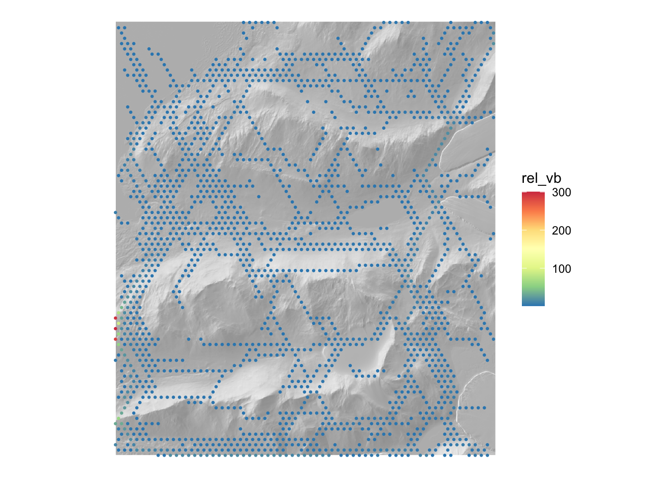
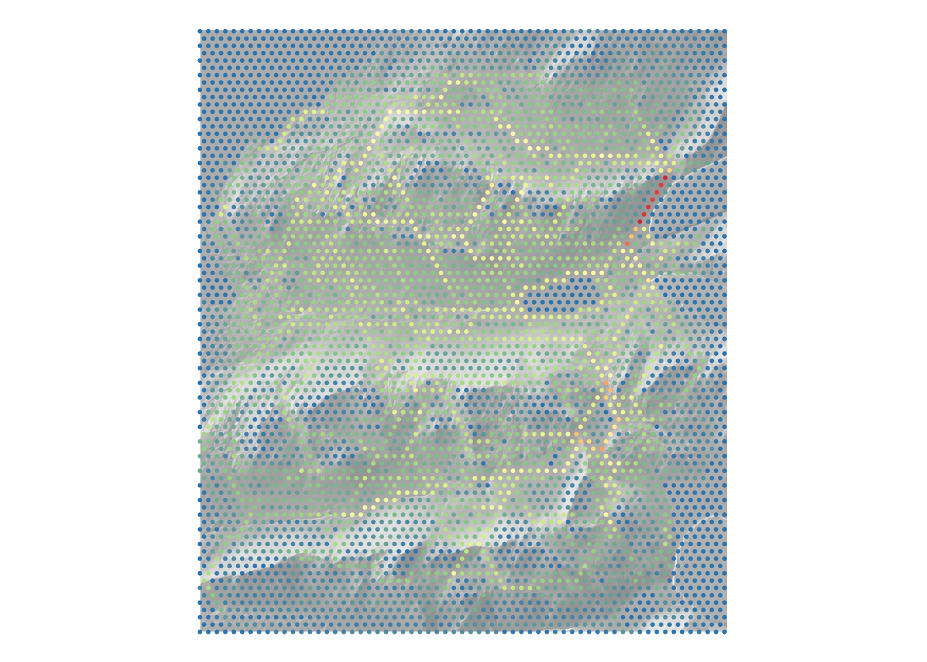
First vertex centrality, where it is relatively simple to colour vertices by their centrality.

hillshade_basemap +
  geom_sf(data = Gsp |> get_graph_as_point_layer() |> filter(log_rel_vb > 0), 
          aes(colour = rel_vb), size = 0.5) +
  scale_colour_distiller(palette = "Spectral")

Edge centrality is fiddlier to map (because of how the linewidth aesthetic works).

hillshade_basemap +
  geom_sf(data = Gsp |> get_graph_as_line_layer() |> filter(log_rel_eb > 0) |> mutate(lwd = rel_eb / 100),
          aes(linewidth = lwd)) +
  scale_linewidth_identity(breaks = 0:5 * 50, labels = format(0:5 * 50, scientific = FALSE),
                           guide = "legend", name = "Edge betweenness")

From which we deduce… there is a ‘shortcut’ around the eastern (to the left…) end of the northernmost (bottom…) ridge which the shortest path function is finding.

TODO: Check if this is an appropriate study area…

Restricting the length of shortest paths

It is possible to restrict shortest paths to a maximum length in terms of the cost attribute used to calculate path lengths, which in our case is hours. Intuitively if the longest hike ‘segments’ undertaken are (say) 3 hours, then restricting shortest paths in this way might make sense. So…

vb <- betweenness(G, weights = E(G)$cost, cutoff = 3) + 1
Gsp <- G |>
  set_vertex_attr("betweenness", value = vb)

hillshade_basemap +
  geom_sf(data = Gsp |> get_graph_as_point_layer(), aes(colour = betweenness), size = 0.5) +
  scale_colour_distiller(palette = "Spectral", guide = "none")

This more local focus identifies more vertices as being on shortest paths