library(dplyr)
library(tidyr)
library(stringr)
library(here)
library(sf)
library(terra)
library(tmap)
library(ggplot2)
library(ggpubr)
library(minpack.lm)Estimating a hiking function
A work in progress…
Update History
| Date | Changes |
|---|---|
| 2024-09-26 | Added an executive summary. |
| 2024-07-22 | Added variables to hex bin filter method. |
| 2024-07-19 | Added nlsLM estimation of models. |
| 2024-07-17 | Initial post. |
TL;DR Executive summary
This notebook provides a useful overview of the process of estimating a hiking function from the GPS data but IS SUPERSEDED by this notebook.
src_folder <- str_glue("{here()}/_data/GPS-1516Season-MiersValley")
tgt_folder <- str_glue("{here()}/_data/cleaned-gps-data")
all_traces <- st_read(str_glue("{tgt_folder}/all-gps-traces.gpkg"))
Reading layer `all-gps-traces' from data source
`/Users/david/Documents/work/mwlr-tpm-antarctica/antarctica/_data/cleaned-gps-data/all-gps-traces.gpkg'
using driver `GPKG'
Simple feature collection with 112216 features and 26 fields
Geometry type: POINT
Dimension: XY
Bounding box: xmin: 352183.3 ymin: -1254631 xmax: 364874.4 ymax: -1240066
Projected CRS: WGS 84 / Antarctic Polar StereographicNow look at the slope-speed plots
If we first make a crude estimate using geom_smooth on all the data we can start to appreciate the challenge
ggplot(all_traces, aes(x = slope_h, y = speed_km_h)) +
  geom_point(alpha = 0.25, size = 0.5) +
  geom_smooth() +
  theme_minimal()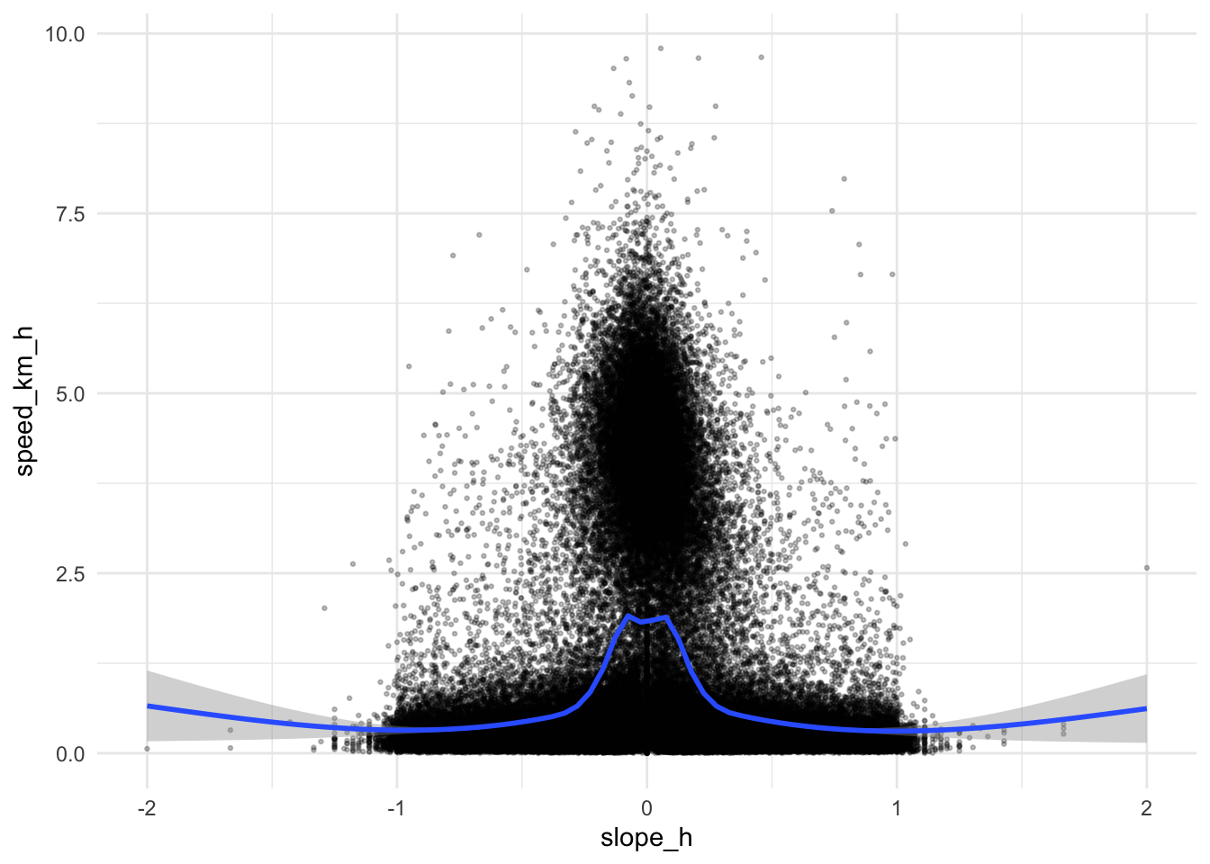
While the result is somewhat bell-shaped as we might hope, there are a lot of fixes that seem unlikely to be related to movement from place to place, rather they are ‘milling about’ in place - such as at basecamp, at experiment sites, at rest stops, etc.
We can of course fit a curve of desired functional form. In the relevant literature, there are essentially two functional forms, exponential, in Waldo Tobler’s original formulation1, given by \[ v=6e^{-3.5\|{s+0.05}\|} \] which gives hiking speed \(v\) in km/h for a slope (given as rise over run) \(s\). This function has subsequently modified by others.2
Other work3 yields speeds essentially Gaussian with respect to slope centred at slight downward slopes, i.e.
\[ v = ae^{-b(s+c)^2} \]
We can explicitly fit such functional forms to the data using the nlsLM function from the minpack.lm package:
# Tobler-like
mod_tobler <- nlsLM(speed_km_h ~ a * exp(-b * abs(slope_h + c)), data = all_traces,
                    start = c(a = 5, b = 3, c = 0.05))
# Gaussian
mod_gauss <- nlsLM(speed_km_h ~ a * dnorm(slope_h, m, s), data = all_traces,
                   start = c(a = 5, m = 0, s = 0.5))
# Student's t (for heavier tails)
mod_students_t <- nlsLM(speed_km_h ~ a * dt((slope_h + m), d), data = all_traces,
                   start = c(a = 5, m = 0, d = 0.001))
Note that we use the probability density functions dnorm and dt here for convenience of parameterisation. It is easier to revert to base R plotting to get a feel for what these look like:
# a non spatial version of the data for plotting - which it is convenient to
gps_data <- all_traces |>
  st_drop_geometry() |>
  select(slope_h, speed_km_h)

s <- -200:200 / 100
slopes <- data.frame(slope_h = s)
plot(gps_data, col = "lightgray", cex = 0.5)
lines(s, predict(mod_tobler, slopes), col = "red", lwd = 2)
lines(s, predict(mod_gauss, slopes), col = "blue", lwd = 2)
lines(s, predict(mod_students_t, slopes), col = "forestgreen", lwd = 2)
legend("topright", legend = c("Tobler", "Gaussian", "Student's t"),
       col = c("red", "blue", "forestgreen"), lwd = 2, lty = 1)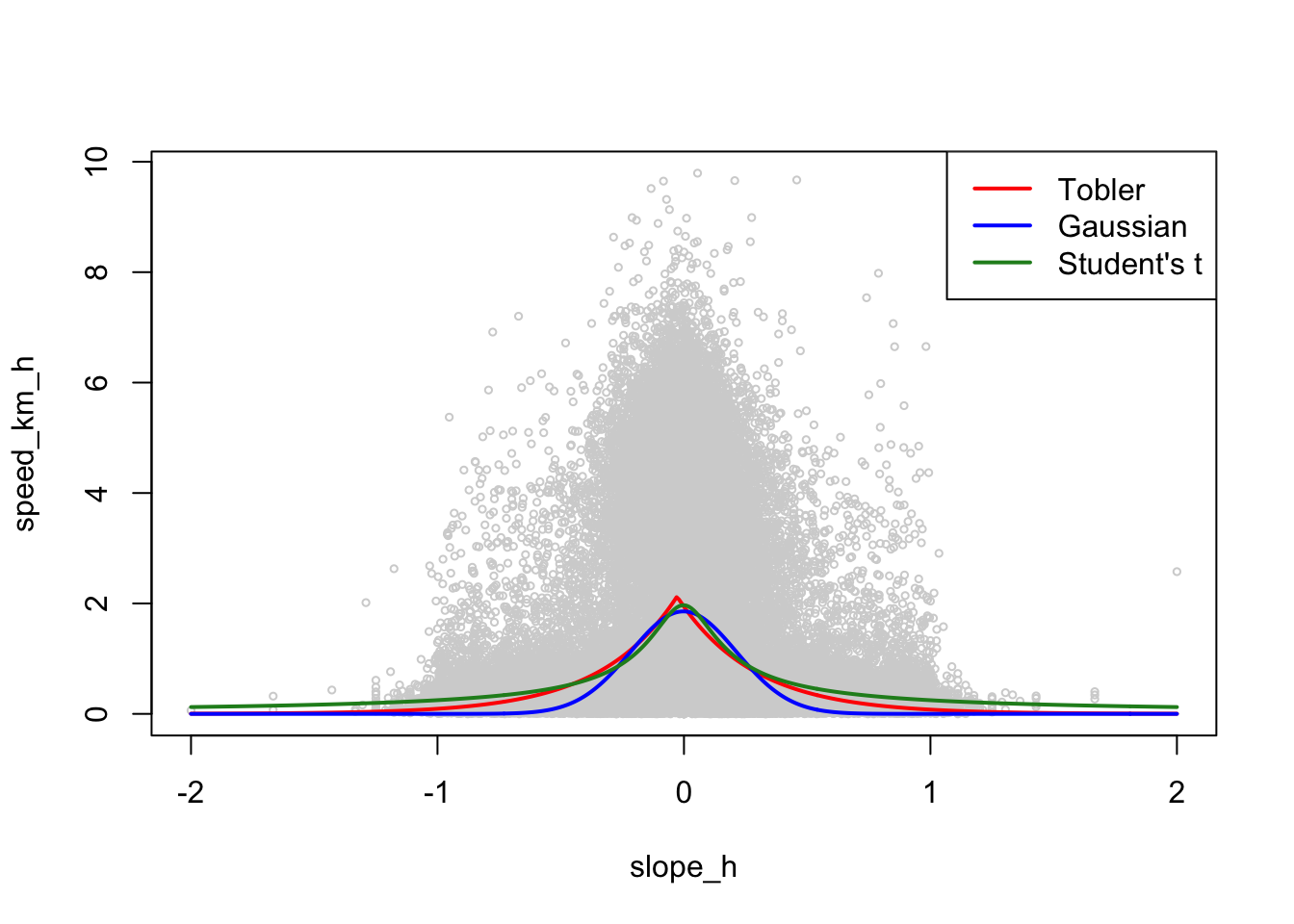
That’s the process… but we need to apply it to filtered data to get closer to a reasonable outcome. Wrap the model-building in convenience functions:
get_tobler_hiking_function <- function(df) {
  nlsLM(speed_km_h ~ a * exp(-b * abs(slope_h + c)), data = df,
        start = c(a = 5, b = 3, c = 0.05))
}

get_gaussian_hiking_function <- function(df) {
  nlsLM(speed_km_h ~ a * dnorm(slope_h, m, s), data = df,
        start = c(a = 5, m = 0, s = 0.5))
}

get_students_t_hiking_function <- function(df) {
  nlsLM(speed_km_h ~ a * dt((slope_h + m), d), data = df,
        start = c(a = 5, m = 0, d = 0.001))
}
Cleaning the data to get a better hiking function
There are a number of features in the data that might allow us to exclude such data from consideration. We examine three below:
- Only consider an ‘upper bound’ on the distribution, say the 90th percentile of
speed_km_hrelative to a given slope - Remove fixes where the density of fixes is high since these may relate to base camp sites, etc.
- Remove fixes with high turn angles, since these may relate to where the data suggest a lot of ‘milling about’
We look at each of these below.
Upper bound of the distribution
If we only consider speed estimates at or close to the upper bound of the data, then we are removing all the milling about data:
d90 <- gps_data |>
  mutate(slope_h = round(slope_h, 2)) |>
  group_by(slope_h) |>
  summarise(speed_km_h = quantile(speed_km_h, 0.9)) |>
  ungroup()

mod_tobler <- get_tobler_hiking_function(d90)
mod_gauss <- get_gaussian_hiking_function(d90)
mod_students_t <- get_students_t_hiking_function(d90)

plot(gps_data, col = "lightgray", cex = 0.5,
     main = "Hiking functions from 90th percentile speeds")
points(d90, cex = 0.5)
lines(s, predict(mod_tobler, slopes), col = "red", lwd = 2)
lines(s, predict(mod_gauss, slopes), col = "blue", lwd = 2)
lines(s, predict(mod_students_t, slopes), col = "forestgreen", lwd = 2)
legend("topright", legend = c("Tobler", "Gaussian", "Student's t"),
       col = c("red", "blue", "forestgreen"), lwd = 2, lty = 1)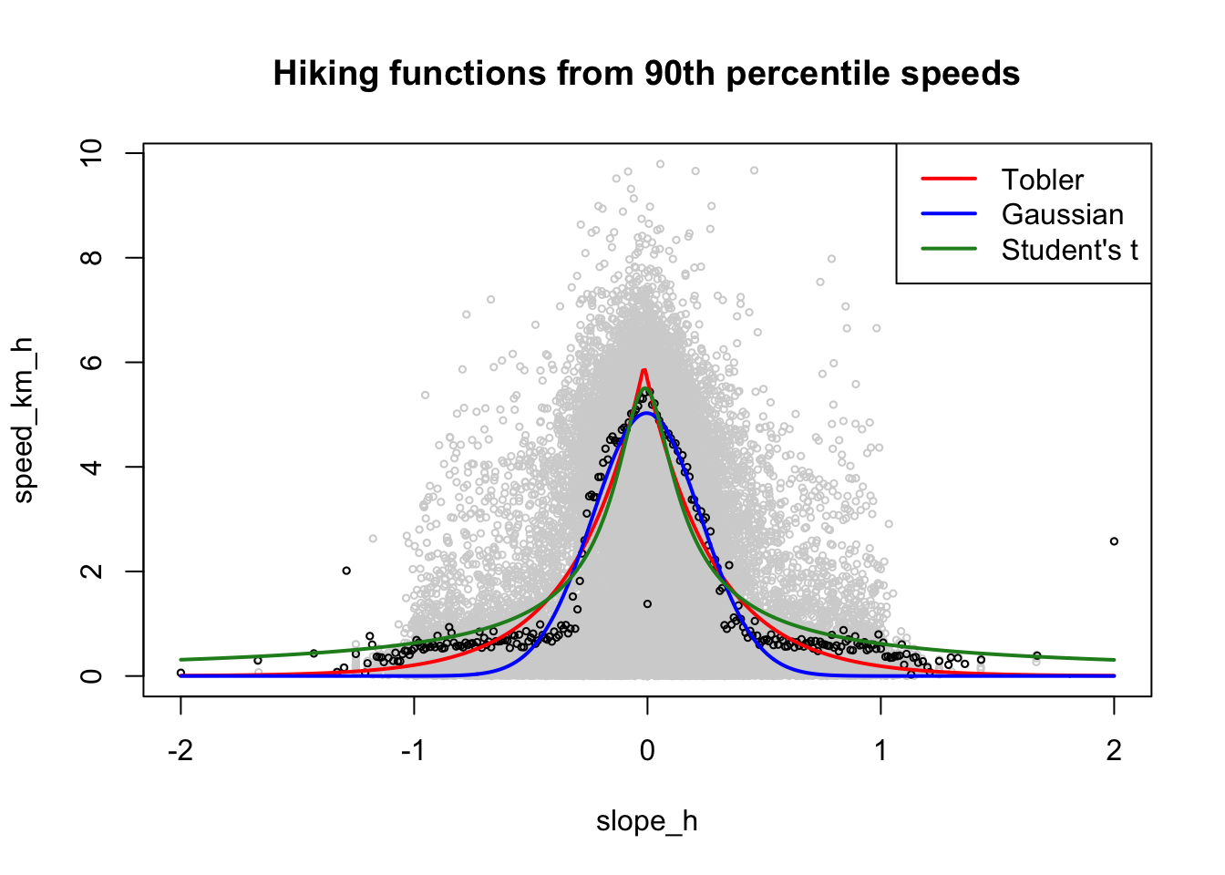
Based on residual sum-of-squares, the Tobler-like function is the best fit in this case (although the differences are small). In this particular case, the paramterisation is strikingly similar to Tobler’s
summary(mod_tobler)
Formula: speed_km_h ~ a * exp(-b * abs(slope_h + c))

Parameters:
  Estimate Std. Error t value Pr(>|t|)
a 5.950260   0.141452  42.065  < 2e-16 ***
b 3.399181   0.114934  29.575  < 2e-16 ***
c 0.014756   0.004926   2.995  0.00302 **
---
Signif. codes:  0 '***' 0.001 '**' 0.01 '*' 0.05 '.' 0.1 ' ' 1

Residual standard error: 0.5403 on 249 degrees of freedom

Number of iterations to convergence: 4
Achieved convergence tolerance: 1.49e-08
Giving us \(v = 5.95e^{-3.39\|s+0.0147\|}\), which only differs much from Tobler’s proposed formula by the offset from 0 slope, which is reduced from 0.05 to 0.0147.
Note that by choosing a different quantile than the 90th percentile we can vary the speeds predicted by a model produced in this way.
Filtering by densely travelled locations
The idea here is that densely travelled locations are near base camps and similar sites, and not where scientists are ‘on the move’. The approach below uses hex binning to find densely trafficked areas and exclude fixes in those areas.
hexes <- all_traces |>
  st_make_grid(cellsize = 60, square = FALSE, what = "polygons") |>
  st_as_sf(crs = st_crs(all_traces)) |>
  rename(geom = x) |>
  st_join(all_traces |> mutate(id = row_number()), left = FALSE) |>
  group_by(geom) |>
  summarise(n = n(), n_persons = n_distinct(name)) |>
  select(n, n_persons) |>
  ungroup() |>
  mutate(density = n / n_persons)
Map with tmap (greater flexibility on the classification scheme)
tm_shape(hexes |> pivot_longer(cols = c(n, n_persons, density))) +
  tm_fill(col = "value", style = "quantile", n = 10, palette = "-magma") +
  tm_facets(by = "name", free.scales = TRUE)
But where to cut off the data? Here are boxplots (note log scales) of the number of fixes n, the number of persons, n_persons, and the number of fixes per person, density, associated with each hex.
hexes |>
  pivot_longer(cols = c(n, n_persons, density)) |>
  ggplot() +
  geom_boxplot(aes(y = value)) +
  scale_y_log10() +
  facet_wrap( ~ name, scales = "free_y", ncol = 3) +
  theme_minimal()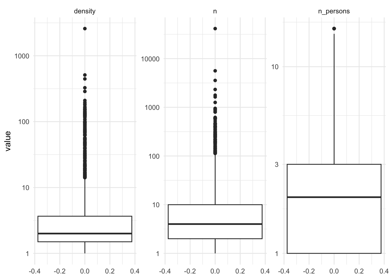
This doesn’t really help! … and it’s not entirely clear that this yields better results!
d_hexes <- all_traces |>
  st_join(hexes) |>
  filter(n < 26) |>
  filter(density < 7.5) |>
  filter(n_persons < 5) |>
  st_drop_geometry() |>
  select(slope_h, speed_km_h)

mod_tobler <- get_tobler_hiking_function(d_hexes)
mod_gauss <- get_gaussian_hiking_function(d_hexes)
mod_students_t <- get_students_t_hiking_function(d_hexes)

plot(gps_data, col = "lightgray", cex = 0.5,
     main = "Hiking functions from less densely trafficked areas")
points(d_hexes, cex = 0.5)
lines(s, predict(mod_tobler, slopes), col = "red", lwd = 2)
lines(s, predict(mod_gauss, slopes), col = "blue", lwd = 2)
lines(s, predict(mod_students_t, slopes), col = "forestgreen", lwd = 2)
legend("topright", legend = c("Tobler", "Gaussian", "Student's t"),
       col = c("red", "blue", "forestgreen"), lwd = 2, lty = 1)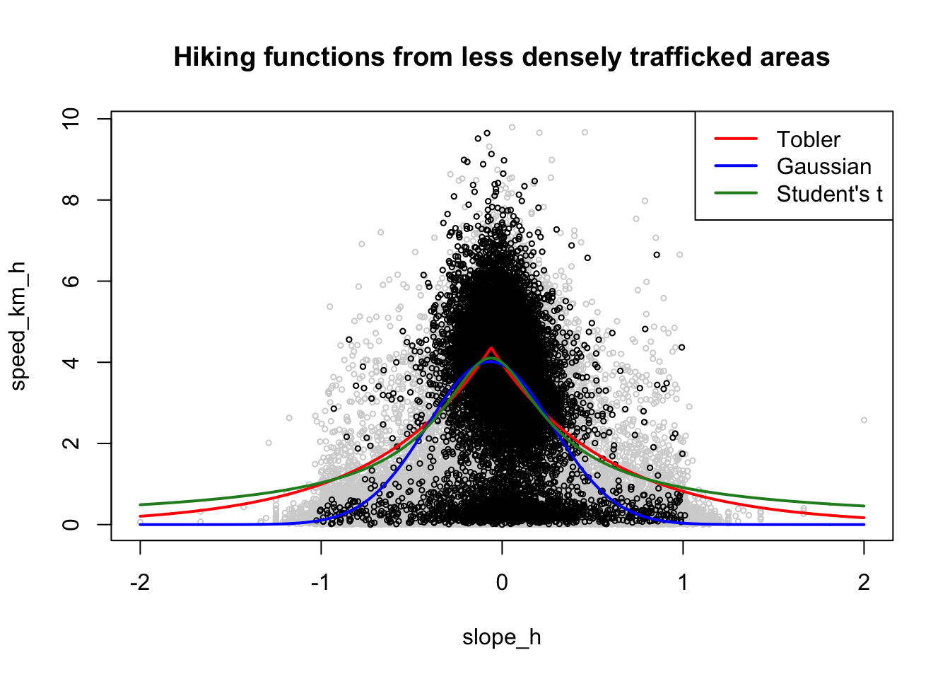
Removing fixes with large turn angles
Again, this is a way to potentially remove data where there is a lot of milling about. As with the density approach, it’s hard to know what is a sensible cutoff. A map of the fixes coloured by turn angle is not necessarily much help:
ggplot(all_traces) +
  geom_sf(aes(colour = turn_angle), size = 0.25)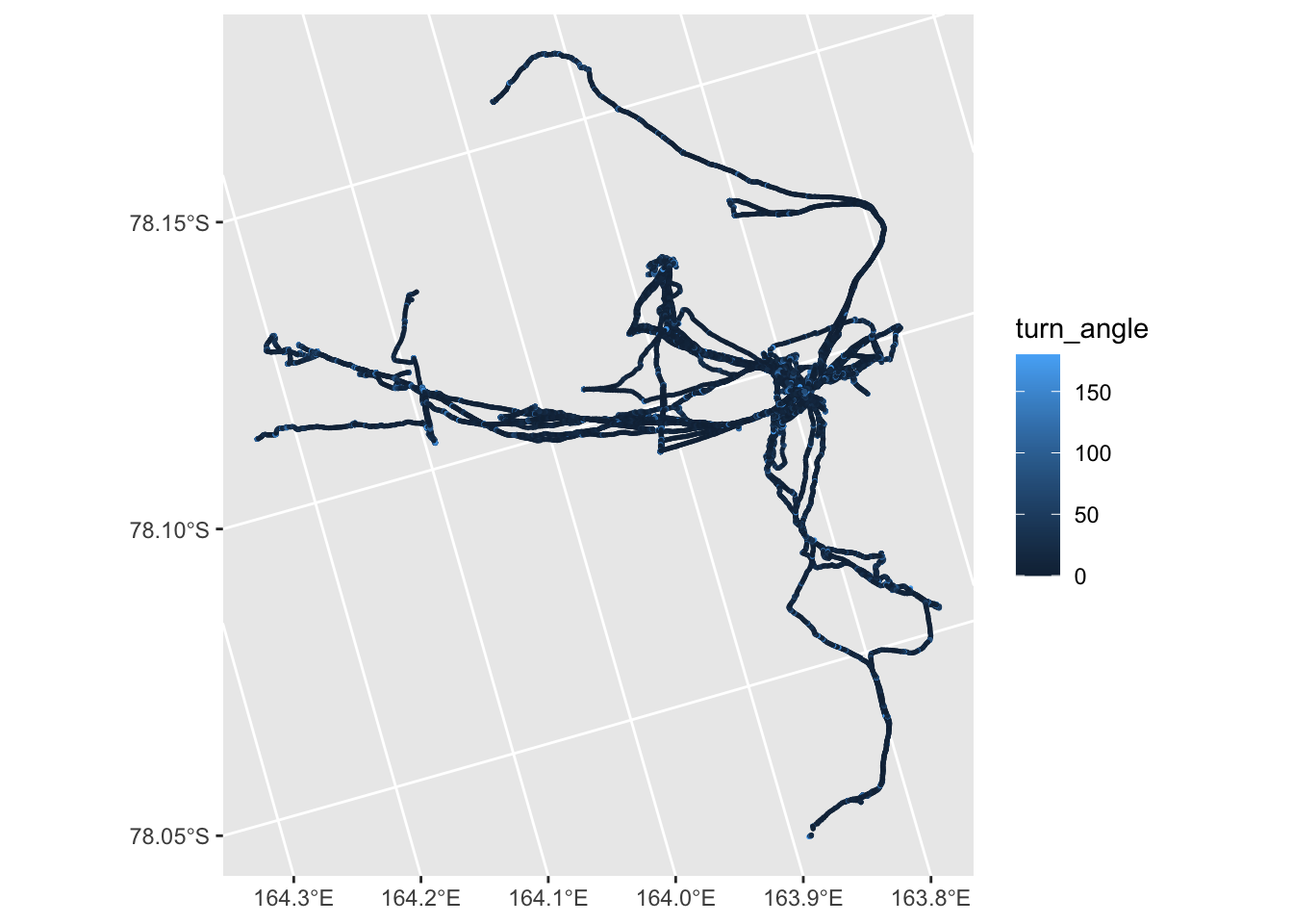
In fact it seems that a rather aggressive seeming filter is needed before base camp and similar areas ‘show through’:
ggplot(all_traces |> filter(turn_angle < 5)) +
  geom_sf(size = 0.2)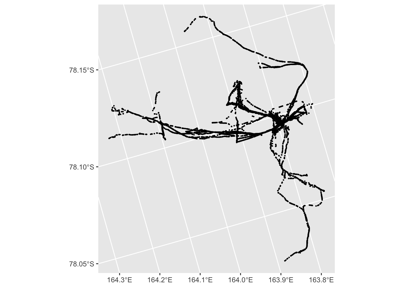
d_low_turn_angle <- all_traces |>
  filter(turn_angle < 5) |>
  st_drop_geometry() |>
  select(slope_h, speed_km_h)

mod_tobler <- get_tobler_hiking_function(d_low_turn_angle)
mod_gauss <- get_gaussian_hiking_function(d_low_turn_angle)
mod_students_t <- get_students_t_hiking_function(d_low_turn_angle)

plot(gps_data, col = "lightgray", cex = 0.5,
     main = "Hiking functions from fixes with low turn angles")
points(d_low_turn_angle, cex = 0.5)
lines(s, predict(mod_tobler, slopes), col = "red", lwd = 2)
lines(s, predict(mod_gauss, slopes), col = "blue", lwd = 2)
lines(s, predict(mod_students_t, slopes), col = "forestgreen", lwd = 2)
legend("topright", legend = c("Tobler", "Gaussian", "Student's t"),
       col = c("red", "blue", "forestgreen"), lwd = 2, lty = 1)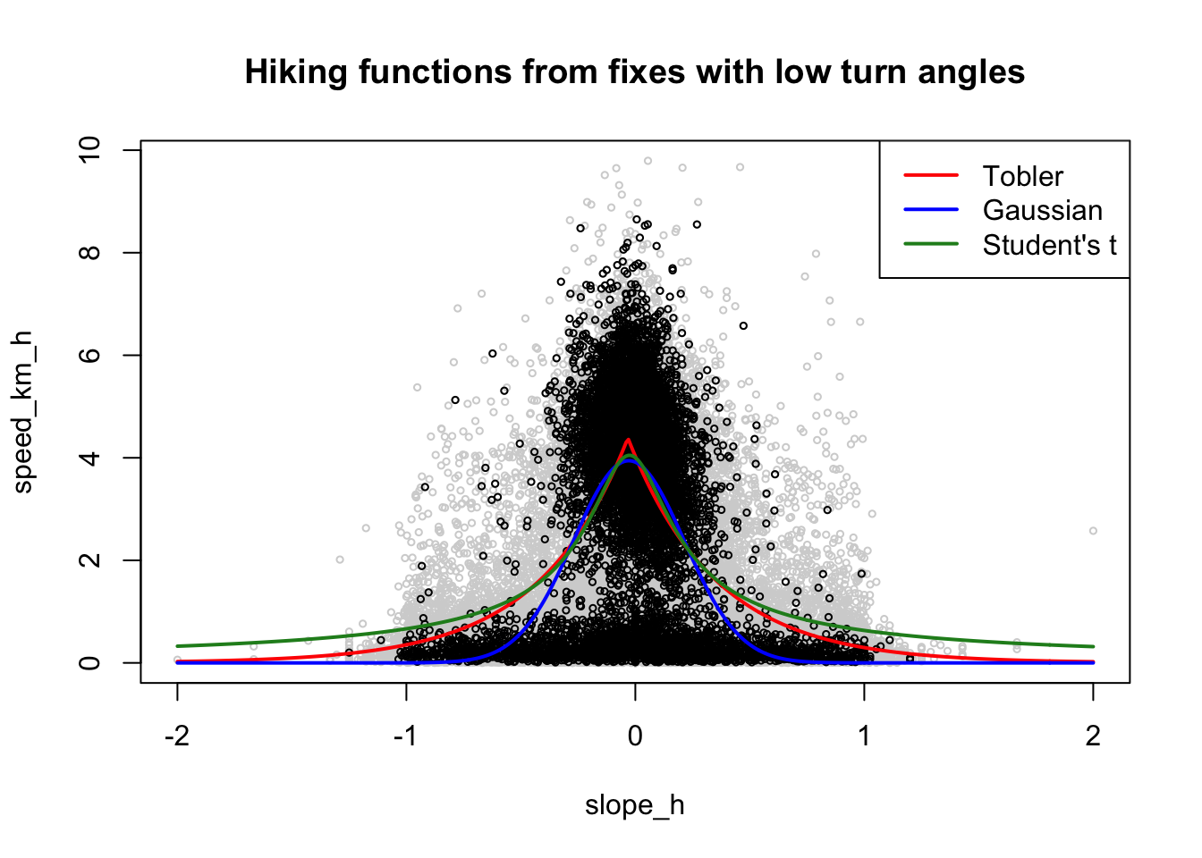
Conclusion
This is still a work in progress…
Footnotes
Tobler WR. 1993. Three Presentations on Geographical Analysis and Modeling: Non-Isotropic Geographic Modeling; Speculations on the Geometry of Geography; and Global Spatial Analysis. Technical Report 93–1. NCGIA Technical Reports. Santa Barbara, CA: National Center for Geographic Information and Analysis.↩︎
See, for example, Márquez-Pérez J, I Vallejo-Villalta and JI Álvarez-Francoso. 2017. Estimated travel time for walking trails in natural areas. Geografisk Tidsskrift-Danish Journal of Geography 117(1) 53–62. doi: 10.1080/00167223.2017.1316212↩︎
Irmischer IJ and KC Clarke. 2018. Measuring and modeling the speed of human navigation. Cartography and Geographic Information Science 45(2). 177–186. doi: 10.1080/15230406.2017.1292150↩︎