Code
library(here)
library(stringr)
library(ggplot2)
library(ggnewscale)
library(whitebox)
library(ggpubr)
library(ggspatial)

source(str_glue("{here()}/scripts/raster-to-graph-functions.R"))Varying resolution and cutoff times in centrality analysis
| Date | Changes |
|---|---|
| 2024-09-26 | Added an executive summary. |
| 2024-09-04 | Added quick analysis of timings. |
| 2024-08-29 | Initial post. |
The key findings are:
This notebook explores the impact of varying the resolution of the hiking network and cutoff times on computation times.
library(here)
library(stringr)
library(ggplot2)
library(ggnewscale)
library(whitebox)
library(ggpubr)
library(ggspatial)
source(str_glue("{here()}/scripts/raster-to-graph-functions.R"))Most of this code is in the previous notebook just wrapped in a couple of loops.
Setup a bunch of folders and base data sets that are unchanged from run to run.
dem_resolution     <- "32m" # 10m also available, but probably not critical
impassable_cost    <- -999  # in the cover-costs file. hat-tip to ESRI
data_folder        <- str_glue("{here()}/_data")
base_folder        <- str_glue("{data_folder}/dry-valleys")
input_folder       <- str_glue("{base_folder}/common-inputs")
output_folder      <- str_glue("{base_folder}/output")
basename           <- str_glue("dry-valleys")
contiguous_geology <- "05"  # use small one '05' for testing

dem_folder         <- str_glue("{data_folder}/dem/{dem_resolution}")
dem_file <- str_glue("{dem_folder}/{basename}-combined-{dem_resolution}-dem-clipped.tif")
extent_file        <- str_glue("{base_folder}/contiguous-geologies/{basename}-extent-{contiguous_geology}.gpkg")
extent             <- st_read(extent_file)

terrain <- rast(dem_file) |>
  crop(extent |> as("SpatVector")) |>
  mask(extent |> as("SpatVector"))
shade <- get_hillshade(terrain) |>
  as.data.frame(xy = TRUE) # this is for plotting in ggplot

hillshade_basemap  <- ggplot(shade) +
  geom_raster(data = shade, aes(x = x, y = y, fill = hillshade), alpha = 0.5) +
  scale_fill_distiller(palette = "Greys", direction = 1) +
  guides(fill = "none") +
  annotation_scale(plot_unit = "m", height = unit(0.1, "cm")) +
  theme_void()

landcover_file     <- str_glue("{input_folder}/{basename}-cover-costs.gpkg")
cover              <- st_read(landcover_file)
resolutions <- c(100, 200)
cutoffs <- c(1:5, -1)
results <- list()
index <- 1
for (resolution in resolutions) {
hex_cell_spacing <- resolution * sqrt(2 / sqrt(3))
# check if we have already made this dataset
hexgrid_file <-
str_glue("{base_folder}/output/{basename}-{contiguous_geology}-{dem_resolution}-hex-grid-{resolution}.gpkg")
if (file.exists(hexgrid_file)) {
xy <- st_read(hexgrid_file)
} else {
xy <- extent |>
st_make_grid(cellsize = hex_cell_spacing, what = "centers", square = FALSE) |>
st_as_sf() |>
rename(geometry = x) |> # shouldsee https://github.com/r-spatial/sf/issues/2429
st_set_crs(st_crs(extent))
coords <- xy |> st_coordinates()
xy <- xy |>
mutate(x = coords[, 1], y = coords[, 2])
xy |>
st_write(str_glue(hexgrid_file), delete_dsn = TRUE)
}
z <- terrain |> terra::extract(xy |> as("SpatVector"), method = "bilinear")
pts <- xy |>
mutate(z = z[, 2]) |>
st_join(cover) |>
filter(!is.na(z), cost != impassable_cost)
graph_file <-
str_glue("{base_folder}/output/{basename}-{contiguous_geology}-{dem_resolution}-graph-hex-{resolution}.txt")
if (file.exists(graph_file)) {
G <- read_graph(graph_file)
} else {
G <- graph_from_points(pts, hex_cell_spacing * 1.1)
write_graph(G, graph_file)
}
# note... for now this uses a default Tobler hiking function
G <- assign_movement_variables_to_graph(G, xyz = pts, impedances = pts$cost)
for (cutoff in cutoffs) {
vb_base_time <- system.time(base_vb <- betweenness(G, cutoff = cutoff))
vb_cost_time <- system.time(cost_vb <- betweenness(G, weights = E(G)$cost, cutoff = cutoff))
base_vb <- scales::rescale(base_vb, to = c(1, 100))
cost_vb <- scales::rescale(cost_vb, to = c(1, 100))
diff_vb <- (cost_vb - base_vb) / (cost_vb + base_vb)
rel_vb <- cost_vb / base_vb
log_rel_vb <- log(rel_vb)
Gsp <- G |>
set_vertex_attr("base_vb", value = base_vb) |>
set_vertex_attr("cost_vb", value = cost_vb) |>
set_vertex_attr("diff_vb", value = diff_vb) |>
set_vertex_attr("rel_vb", value = rel_vb) |>
set_vertex_attr("log_rel_vb", value = log_rel_vb)
results[[index]] <- vertex.attributes(Gsp) |>
as.data.frame() |>
mutate(resolution = resolution, cutoff = cutoff,
vb_base_time = vb_base_time[3],
vb_cost_time = vb_cost_time[3])
index <- index + 1
}
}
results <- bind_rows(results)results <- results |>
mutate(resolution = as.factor(resolution),
cutoff = as.factor(cutoff)) |>
mutate(cutoff = if_else(cutoff == -1, "None", cutoff))hillshade_basemap +
geom_point(data = results |> filter(resolution == 100),
aes(x = x, y = y, colour = cost_vb), size = 0.09) +
scale_colour_viridis_c(option = "A", direction = -1) +
coord_equal() +
facet_wrap( ~ cutoff, nrow = 3, labeller = label_both) +
ggtitle("Hiking network nominal resolution: 100m")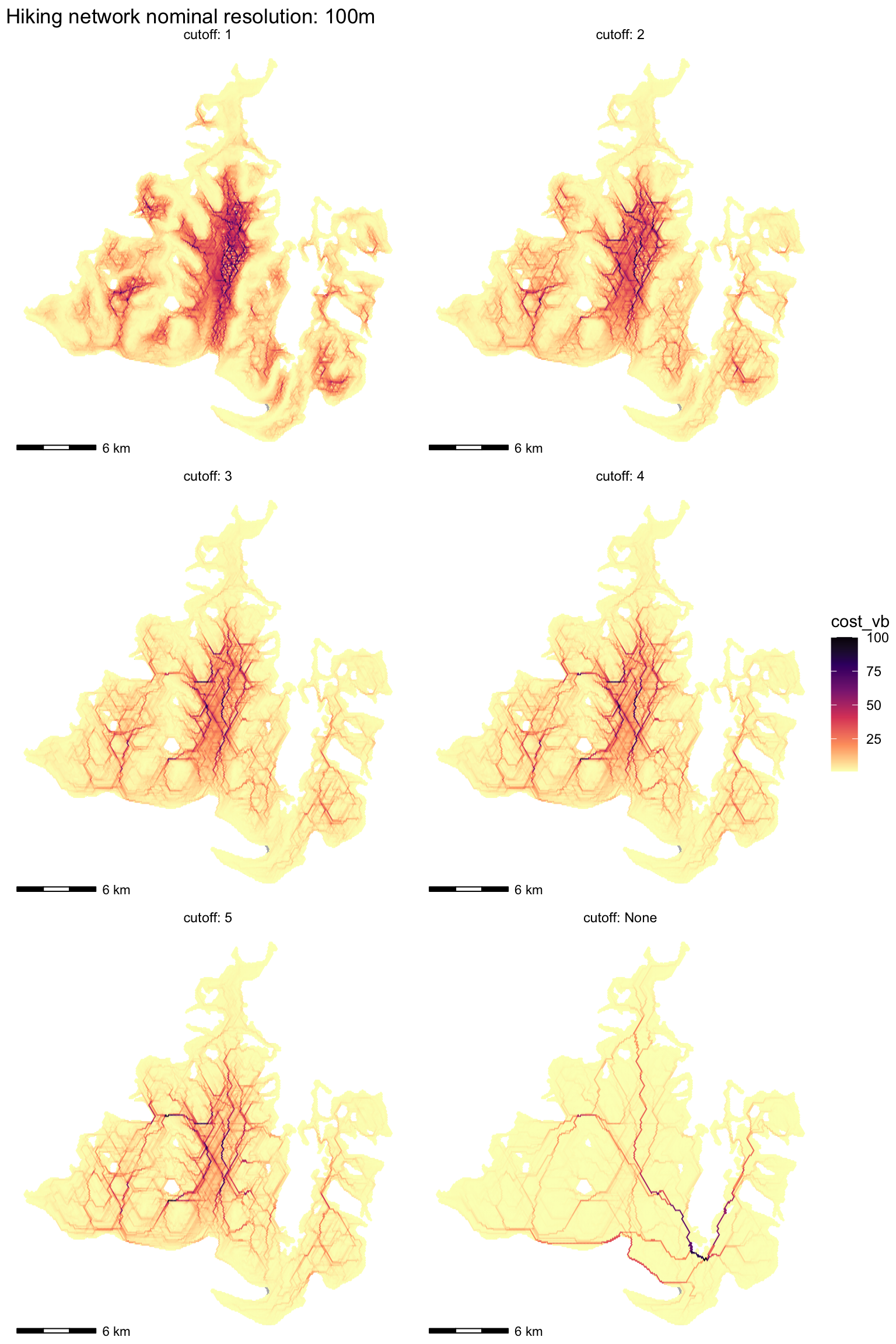
hillshade_basemap +
  geom_point(data = results |> filter(resolution == 200),
             aes(x = x, y = y, colour = cost_vb), size = 0.2) +
  scale_colour_viridis_c(option = "A", direction = -1) +
  coord_equal() +
  facet_wrap( ~ cutoff, nrow = 3, labeller = label_both) +
  ggtitle("Hiking network nominal resolution: 200m")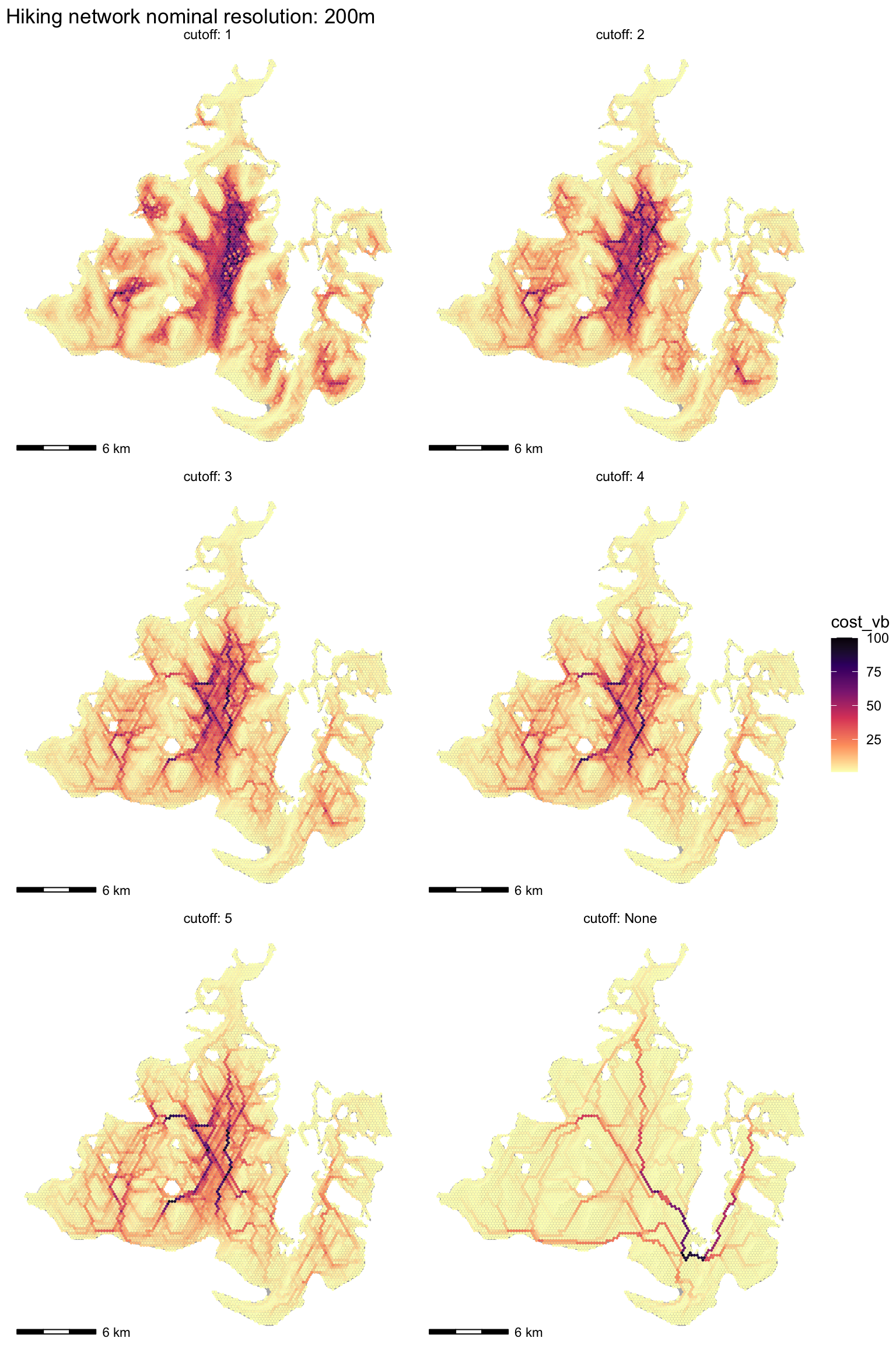
Export these results for interactive examination in QGIS.
[NOT RUN]
for (c in cutoffs) {
  for (r in resolutions) {
    results |> filter(cutoff == c, resolution == r) |>
      st_as_sf(coords = c("x", "y")) |>
      st_set_crs(st_crs(extent)) |>
      st_write(
        str_glue("{output_folder}/{basename}-{contiguous_geology}-{dem_resolution}-betweenness-{r}-{c}.gpkg"),
        delete_dsn = TRUE)
  }
}The timing for this small area of interest at these resolutions and cutoff times are tabulated below.
df <- results |>
  select(resolution, vb_base_time, vb_cost_time, cutoff) |>
  distinct() |>
  pivot_longer(cols = c(vb_base_time, vb_cost_time))

ggplot(df) +
  geom_col(aes(x = cutoff, y = value, group = resolution, fill = resolution), position = "dodge") +
  xlab("Betweenness calculation est. hiking time cutoff") +
  ylab("Time, sec") +
  theme_minimal()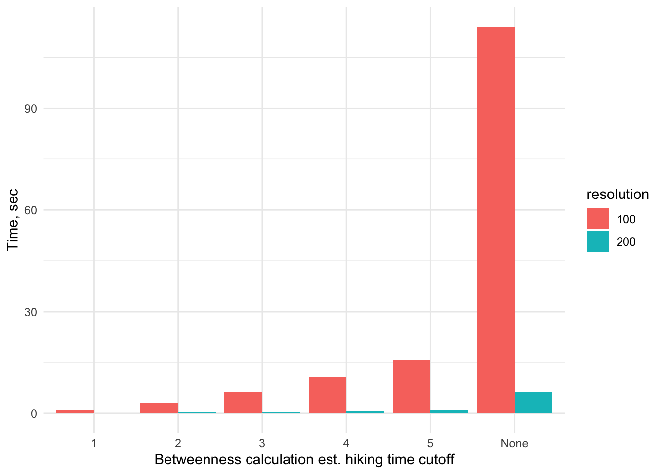
This confirms that the time to perform betweenness centrality estimation increases with the square of the number of vertices in the network. The finer resolution network (100m) has four times as many nodes, and analysis takes around 16 times longer (>15 seconds vs ~ 1 second in the cutoff = 5 case).
When no cutoff time is used, the betweenness calculation takes much longer. It is clear from the maps above that the no cutoff case identifies ‘arterials’ although it is unclear that this is the most relevant concern for expected environmental impacts.
Further analysis of larger networks (the networks for the largest contiguous region are about 10 times larger than this one) confirms this result, with comparable analyses taking ~100 times longer, which on the computer used (an M2 Mac Mini) translates to several hours compute time for the most extensive betweenness estimation at 100m resolution.
These results suggest that it is important to settle on a resolution and cutoff distance judged appropriate for ongoing work to avoid costly repetition of sometimes time-consuming analysis. It is almost certainly preferable to apply some cutoff estimated hiking time to the calculation in any case.