Betweenness centrality based on a limited set of locations

Using shortest paths and minimum spanning trees

Update History

Date	Changes
2024-09-19	Detailed the commentary.
2024-09-16	Initial post.

This notebook explores developing the betweenness centrality networks/risk maps based on a known set of most often used origins and destinations. The idea would be to supply a list of locations with associated weightings, where for example base camp might be (say) 25, some once-visited sampling locations might be ‘1’, repeat-visit experimental sites might be 5. Betweenness is then based on all shortest paths among these sites weighted by those numbers.

As an extension it might be possible to use outputs from this to propose a low impact network of routes to use for an expedition.

library(here)
library(stringr)
library(ggplot2)
library(ggnewscale)
library(ggspatial)
library(hrbrthemes)
library(spatstat)
library(purrr)
library(igraph)

source(str_glue("{here()}/scripts/raster-to-graph-functions.R"))

Setting up the data sets and folders

This is similar to many previous notebooks.

dem_resolution     <- "32m" # 10m also available, but probably not critical
impassable_geology <- "ice"
data_folder        <- str_glue("{here()}/_data")
base_folder        <- str_glue("{data_folder}/dry-valleys")
input_folder       <- str_glue("{base_folder}/common-inputs")
output_folder      <- str_glue("{base_folder}/output")
basename           <- str_glue("dry-valleys")
contiguous_geology <- "05"  # use small one '05' for testing

dem_folder         <- str_glue("{data_folder}/dem/{dem_resolution}")
dem_file           <- str_glue("{dem_folder}/{basename}-combined-{dem_resolution}-dem-clipped.tif")
extent_file        <- str_glue("{base_folder}/contiguous-geologies/{basename}-extent-{contiguous_geology}.gpkg")
extent             <- st_read(extent_file)

terrain <- rast(dem_file) |>
  crop(extent |> as("SpatVector")) |>
  mask(extent |> as("SpatVector"))
shade <- get_hillshade(terrain) |>
  as.data.frame(xy = TRUE) # this is for plotting in ggplot

hillshade_basemap  <- ggplot(shade) +
  geom_raster(data = shade, aes(x = x, y = y, fill = hillshade), alpha = 0.5) + 
  scale_fill_distiller(palette = "Greys", direction = 1) +
  guides(fill = "none") +
  annotation_scale(plot_unit = "m", height = unit(0.1, "cm")) +
  theme_void()

geologies_file     <- str_glue("{data_folder}/ata-scar-geomap-geology-v2022-08-clipped.gpkg")

Also similar is building or retrieving the graph representation of the terrain.

resolution <- 150

hex_cell_spacing <- resolution * sqrt(2 / sqrt(3))
# check if we have already made this dataset
hexgrid_file <- str_glue("{base_folder}/output/{basename}-{contiguous_geology}-{dem_resolution}-hex-grid-{resolution}.gpkg")
if (file.exists(hexgrid_file)) {
  xy <- st_read(hexgrid_file)
} else {
  xy  <- extent |>
    st_make_grid(cellsize = hex_cell_spacing, what = "centers", square = FALSE) |>
    st_as_sf() |>
    rename(geometry = x) |>
    st_set_crs(st_crs(extent))
  coords <- xy |> st_coordinates()
  xy <- xy |>
    mutate(x = coords[, 1], y = coords[, 2])
  xy |>
    st_write(str_glue(hexgrid_file), delete_dsn = TRUE)
}

z <- terrain |> 
  terra::extract(xy |> as("SpatVector"), method = "bilinear")

pts <- xy |>
  mutate(z = z[, 2])

# remove any NAs that might result from interpolation or impassable terrain
# NAs tend to occur around the edge of study area
cover <- st_read(geologies_file) |>
  dplyr::select(POLYGTYPE) |> 
  rename(terrain = POLYGTYPE)

pts <- pts |>
  st_join(cover) |>
  filter(!is.na(z), terrain != impassable_geology)

graph_file <-   
  str_glue("{base_folder}/output/{basename}-{contiguous_geology}-{dem_resolution}-graph-hex-{resolution}.txt") 
if (file.exists(graph_file)) {
  G <- read_graph(graph_file) 
} else {
  G <- graph_from_points(pts, hex_cell_spacing * 1.1)
  write_graph(G, graph_file)
}

G <- assign_movement_variables_to_graph_2(G, xyz = pts, terrain = pts$terrain)
V(G)$id <- 1:length(G)
cost_cutoff <- 0.5 * resolution / 100
G <- delete_edges(G, E(G)[which(E(G)$cost > cost_cutoff)]) |>
  largest_component(mode = "strong")

remaining_nodes <- V(G)$id
pts <- pts |> slice(remaining_nodes)

Make a bunch of origin locations

Use spatstat to make a set of random locations that are at least somewhat spaced apart.

origin_pts <- rSSI(2000, n = 20, win = as.owin(extent)) |> 
  st_as_sf() |> 
  st_set_crs(st_crs(extent)) |> 
  slice(-1) |> 
  dplyr::select(-label)
# get the sequence numbers of thes in the pts data
origin_is <- origin_pts |>
  st_nearest_feature(pts)
# make up a point dataset of these origins with randomly assigned importance
origin_vs <- pts |>
  mutate(id = row_number()) |>
  slice(origin_is) |>
  mutate(importance = sample(1:25, n(), replace = TRUE, prob = 25:1))

Connect them all in various ways

While doing so, we accumulate how often they appear on shortest paths.

There are a couple of key issues to note here:

• The weights parameter referenced if using all all_shortest_paths MUST NOT be equal across all edges. If it is, then given the uniformity of the underlying lattice there is likely to be a combinatorial explosion as all the many equal shortest paths between every pair of sites are calculated.
• The first version (NOT USED) considers potential multiple shortest paths between sites and is much slower because of the nested iteration and relatively complicated join process along with the down-weighting of vertices when more than one path is found between two sites. This is almost certainly an unnecessary detail.

result <- data.frame(v = V(G) |> 
                       as.vector() |> 
                       as.character(), 
                     betweenness = 0)
for (i in 1:nrow(origin_vs)) {
  for (j in 1:nrow(origin_vs)) {
    if (i != j) {
      ASP <- all_shortest_paths(G, origin_vs$id[i], origin_vs$id[j], 
                                weights = edge_attr(G, "cost"))
      n_shortest_paths <- length(ASP$vpaths)
      result <- result |> 
        left_join(ASP$vpaths |>
                    lapply(as.vector) |>
                    reduce(c) |>
                    table() |>
                    as.data.frame() |>
                    mutate(v = as.character(Var1)) |>
                    dplyr::select(-Var1), by = "v") |>
        mutate(Freq = replace_na(Freq, 0)) |>
        mutate(betweenness = 
                 betweenness + Freq / n_shortest_paths *
                 origin_vs$importance[i]) |>
        dplyr::select(-Freq)
    }
  }
}
G <- G |> set_vertex_attr("sp_betweenness", value = result$betweenness)

• The second version is much quicker, but is an approximation to the extent that it ignores competing equal shortest paths, but instead chooses one at random (or by whatever means igraph makes this choice). Note that unless two paths are exactly the same total cost then the much slower unused version of the code will still, in effect, pick the shorter path, when in fact ‘on the ground’ either might be just as likely to be selected. First up, we use it calculate all sites to all sites shortest paths and overlay those.

# put all vertices on a shortest path to begin
vs_on_shortest_paths <- V(G) |> 
  as.vector()

# make a data frame we can join the results into
for (i in seq_along(origin_vs$id)) {
  # one entry for each appearance on a shortest path
  SP <- shortest_paths(G, origin_vs$id[i], origin_vs$id[-i], weights = edge_attr(G, "cost"))
  new_shortest_paths <- SP$vpath |>
    lapply(as.vector) |>
    reduce(c) |>
    rep(origin_vs$importance[i])
  vs_on_shortest_paths <- vs_on_shortest_paths |>
    c(new_shortest_paths)
}
shortest_path_counts <- vs_on_shortest_paths |>
  table() |>
  as.vector()
G <- set_vertex_attr(G, "sp_betweenness", value = shortest_path_counts - 1)

And map it

spb <- G |> igraph::as_data_frame(what = "vertices")
hillshade_basemap + 
  geom_point(data = spb |> filter(sp_betweenness > 0), 
             aes(x = x, y = y, colour = sp_betweenness),size = 0.25) +
  scale_colour_viridis_c(option = "A", direction = -1) +
  geom_sf(data = origin_vs, aes(size = importance), colour = "black", pch = 1) +
  theme_ipsum_rc()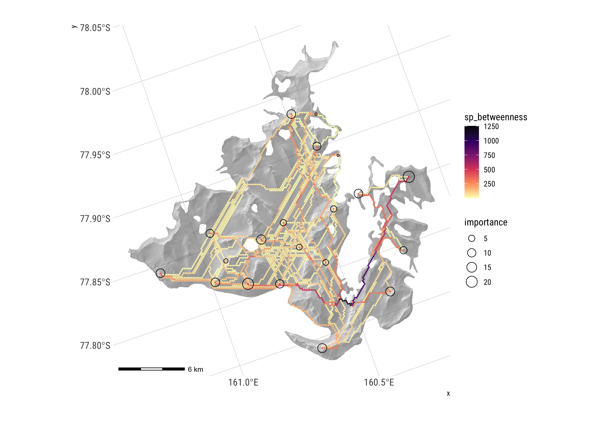

A naive attempt to determine a minimal network

Here, we calculate the distance matrix and determine the greatest minimum distance to a near site across all sites, then construct a network consisting only of connections shorter than this.

dist_m <- distances(G, origin_vs$id, origin_vs$id, weights = edge_attr(G, "cost"))
diag(dist_m) <- max(dist_m)
row_max_min <- dist_m |> apply(MARGIN = 1, FUN = min) |> max()
col_max_min <- dist_m |> apply(MARGIN = 2, FUN = min) |> max()
cutoff <- max(row_max_min, col_max_min)

# hence the connections to be made are given by
which_ijs <- which(dist_m <= cutoff, arr.ind = TRUE)
# and proceed as before
vs_on_shortest_paths <- V(G) |> 
  as.vector()
# make a data frame we can join the results into
for (k in 1:nrow(which_ijs)) {
  i <- which_ijs[k, 1]
  j <- which_ijs[k, 2]
  # one entry for each appearance on a shortest path
  SP <- shortest_paths(G, origin_vs$id[i], origin_vs$id[j], weights = edge_attr(G, "cost"))
  new_shortest_paths <- SP$vpath[[1]] |>
    as.vector() |>
    rep(origin_vs$importance[i])
  vs_on_shortest_paths <- vs_on_shortest_paths |>
    c(new_shortest_paths)
}
shortest_path_counts <- vs_on_shortest_paths |>
  table() |>
  as.vector()
G <- set_vertex_attr(G, "sp_betweenness", value = shortest_path_counts - 1)

And map it

spb <- G |> igraph::as_data_frame(what = "vertices")
hillshade_basemap + 
  geom_point(data = spb |> filter(sp_betweenness > 0), 
             aes(x = x, y = y, colour = sp_betweenness),size = 0.25) +
  scale_colour_viridis_c(option = "A", direction = -1) +
  geom_sf(data = origin_vs, aes(size = importance), colour = "black", pch = 1) +
  theme_ipsum_rc()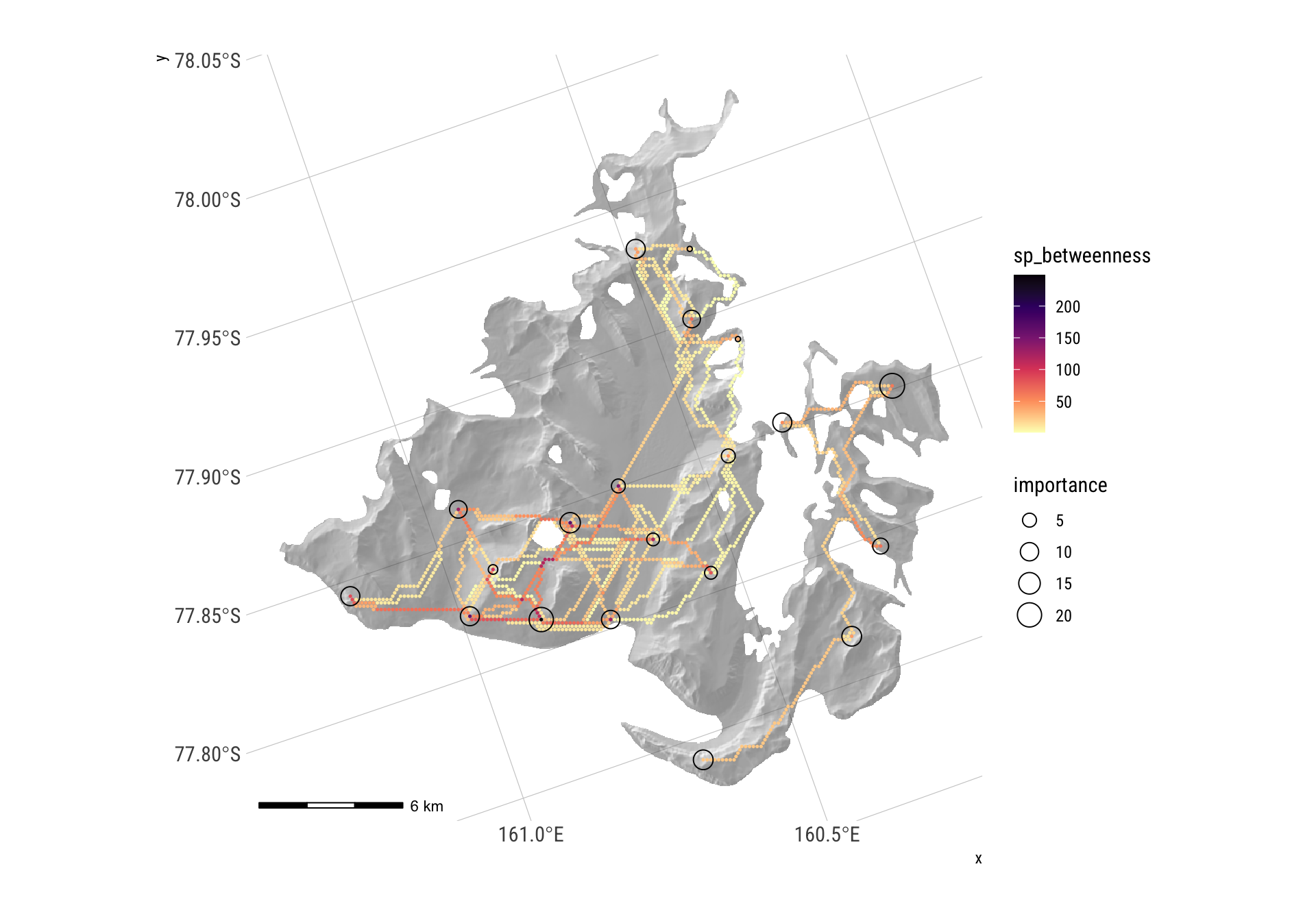

A minimal network connecting all sites

We can use a minimum spanning tree to make a network instead… with one reservation: the minimum spanning tree of a directed graph is not found using algorithms for MSTs on undirected graphs, such as that offered by igraph::mst.

The directed graph equivalent to an MST is called a minimum-cost arborescence or optimal branching.¹ The networkx package in python supports the required algorithms, but igraph does not.

Since the asymmetry in our networks is not extreme, we can approximate a solution in igraph in this case by round tripping the network via an undirected network and back to a directed one.

First the incorrect arborescence…

xs <- vertex_attr(G, "x", V(G)[origin_vs$id])
ys <- vertex_attr(G, "y", V(G)[origin_vs$id])
approx_min_arborescence <- dist_m |> 
  graph_from_adjacency_matrix(mode = "directed", weighted = TRUE) |>
  set_vertex_attr("x", value = xs) |>
  set_vertex_attr("y", value = ys) |>
  mst() # this applies algorithms appropriate to an undirected graph
plot(approx_min_arborescence, 
     vertex.size = 20, edge.arrow.size = .35, 
     xlim = range(xs), ylim = range(ys), rescale = FALSE, asp = 1)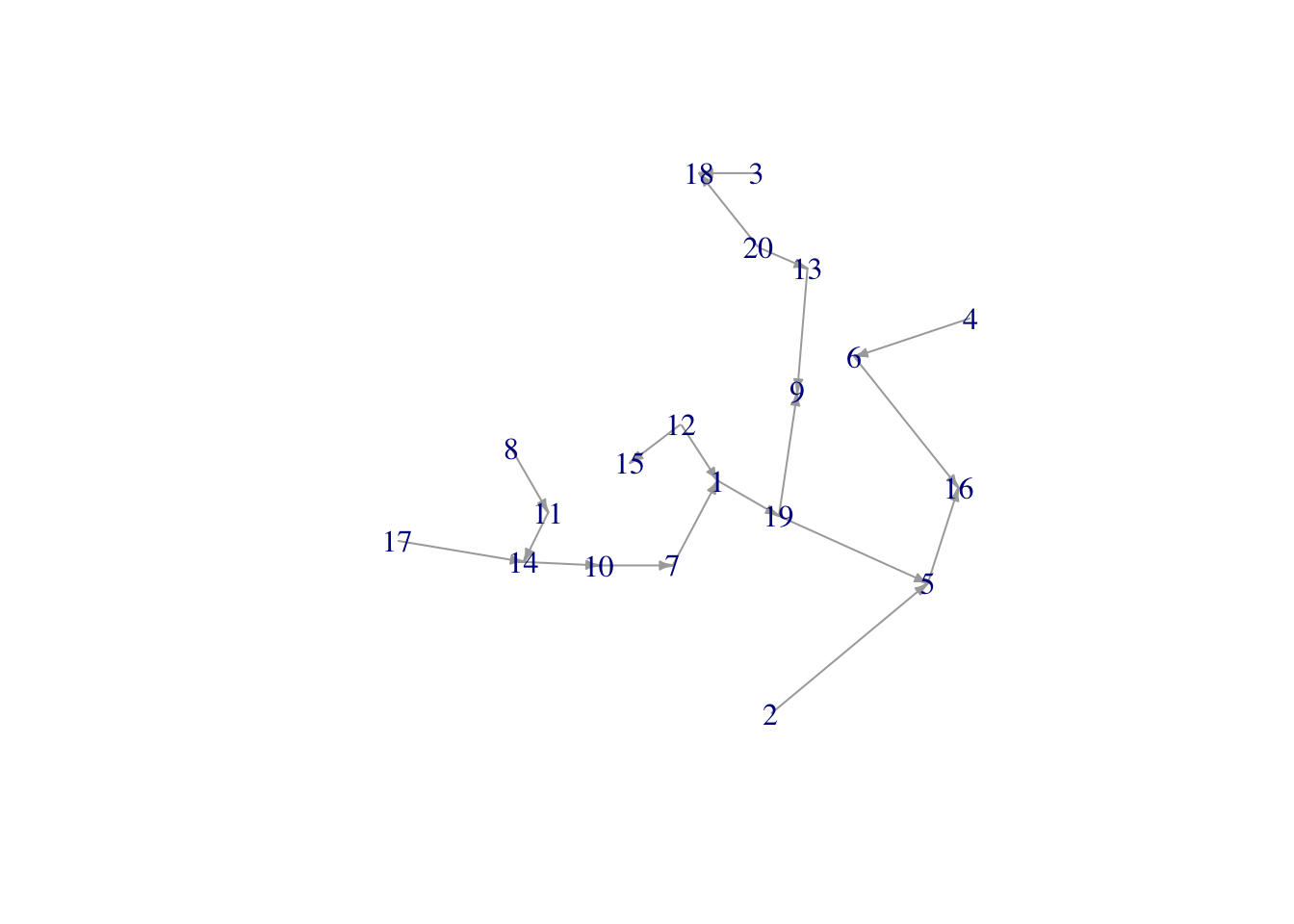

Now round-trip it via an undirected graph. For some reason, I can’t get igraph::as.undirected() to do this, so use matrix representation.

dir_m <- approx_min_arborescence |> as_adjacency_matrix(sparse = FALSE)
undir_m <- ((dir_m + t(dir_m)) > 0)
which_ijs <- which(undir_m, arr.ind = TRUE)

# put all vertices on a shortest path to begin
vs_on_shortest_paths <- V(G) |> 
  as.vector()

# make a data frame we can join the results into
for (k in 1:nrow(which_ijs)) {
  i <- which_ijs[k, 1]
  j <- which_ijs[k, 2]
  # one entry for each appearance on a shortest path
  SP <- shortest_paths(G, origin_vs$id[i], origin_vs$id[j], weights = edge_attr(G, "cost"))
  new_shortest_paths <- SP$vpath[[1]] |>
    as.vector() |>
    rep(origin_vs$importance[i])
  vs_on_shortest_paths <- vs_on_shortest_paths |>
    c(new_shortest_paths)
}
shortest_path_counts <- vs_on_shortest_paths |>
  table() |>
  as.vector()
G <- set_vertex_attr(G, "sp_betweenness", value = shortest_path_counts - 1)

And once more… map it

spb <- G |> igraph::as_data_frame(what = "vertices")
hillshade_basemap + 
  geom_point(data = spb |> filter(sp_betweenness > 0), 
             aes(x = x, y = y, colour = sp_betweenness),size = 0.25) +
  scale_colour_viridis_c(option = "A", direction = -1) +
  geom_sf(data = origin_vs, aes(size = importance), colour = "black", pch = 1) +
  theme_ipsum_rc()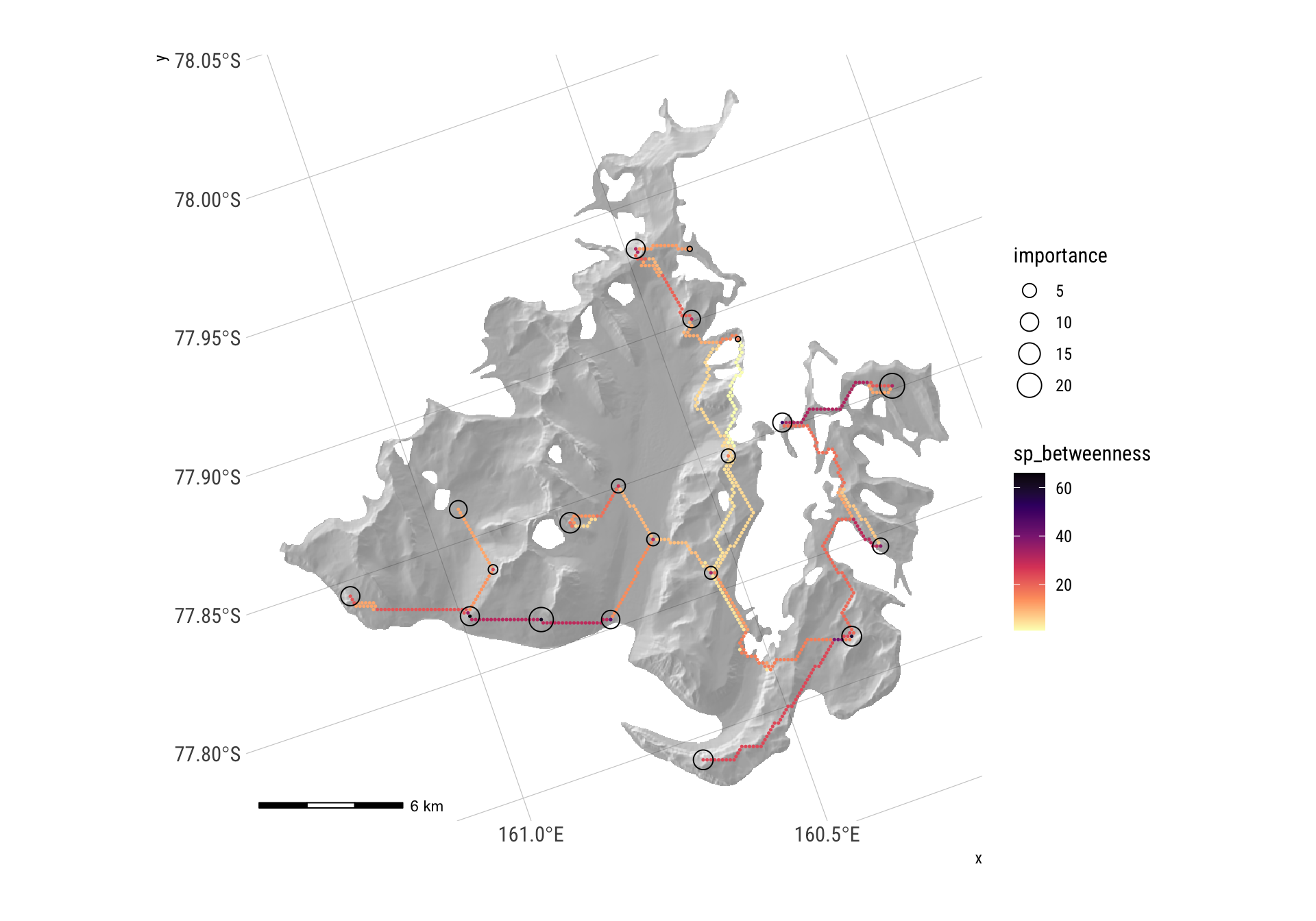

It is interesting to note the total cost of this network and the cost of its longest connection between sites:

edges <- which_ijs |>
  as.data.frame() |>
  mutate(from = origin_vs$id[row], to = origin_vs$id[col]) |>
  mutate(cost = 0) |> 
  dplyr::select(-row, -col)
vertices <- data.frame(
  id = origin_vs$id,
  x = vertex_attr(G, "x", origin_vs$id),
  y = vertex_attr(G, "y", origin_vs$id))
for (k in 1:nrow(edges)) {
  i <- edges$from[k]
  j <- edges$to[k]
  costs = distances(G, i, j, weights = edge_attr(G, "cost"))
  edges$cost[k] <- costs |> as.vector()
}
print(str_glue("Total cost: {sum(edges$cost)}\nHighest cost: {max(edges$cost)}"))

Total cost: 53.1451751235408
Highest cost: 3.06211977831383

Footnotes

1. See this and Korte B and J Vygen. 2018. Spanning Trees and Arborescences. In Combinatorial Optimization: Theory and Algorithms, ed. B Korte and J Vygen, 133–157. Berlin, Heidelberg: Springer. doi:10.1007/978-3-662-56039-6_6.