Refining hiking network construction

Dealing with impassable edges

Author

David O’Sullivan

Published

September 26, 2024

Update History

Date	Changes
2024-09-26	Initial post.

This notebook supersedes some previous work because it handles ‘too steep’ (actually too slow) edges in the network by removing them, and also makes use of the recalculated estimated hiking functions.

Removal of too slow edges is based on an arbitrary threshold such that on a network of nominal resolution 100m (where edges are 107.5m long) if the traversal time is greater than half an hour it is considered impassable and removed from the network. There’s a chicken and egg problem where we have to build the network and add all the vertex and edge attributes before determining which edges to remove. Meanwhile we are unable to store the network reliably due to some issues with the igraph::write_graph functions (note that in general storing graphs is challenging with few reliably implemented and agreed standards—a better approach might be to save vertex and edge data frames. Something to look into).

Code

library(here)
library(stringr)
library(ggplot2)
library(ggnewscale)
library(whitebox)
library(ggpubr)
library(ggspatial)
library(scales)

source(str_glue("{here()}/scripts/raster-to-graph-functions.R"))

Set up folders and some base parameters

The set up of data subfolders under the top level _data folder is largely as before but we now read in the geology (not a cover costs):

Folder	Contents
`dry-valleys/output`	Outputs - primarily the graph and elevation data (as points) with relative movement costs
`contiguous-geologies`	GPKG files `dry-valleys-extent-??.gpkg` with a single contiguous geology polygon per file
`dry-valleys/common-inputs`	Various input layers as needed. Primarily relative landcover costs `*-cover-costs.gpkg`
`dem/10m`	DEM datasets in `raw` and `clipped` (to the Dry Valleys and Skelton basins) and a mosaiced and clipped DEM file `dry-valleys-combined-10m-dem-clipped.tif`
`dem/32m`	DEM datasets in `raw` and `clipped` (to the Dry Valleys and Skelton basins) and a mosaiced and clipped DEM file `dry-valleys-combined-32m-dem-clipped.tif`
`_data`	the geology layer `ata-scar-geomap-geology-v2022-08-clipped.gpkg`

Additionally, the basename for all files is dry-valleys, with DEM resolution used (32m or 10m) and the nominal hiking network resolution (without the m), which is likely to be 100 included in various output files as appropriate.

Code

dem_resolution     <- "32m" # 10m also available, but probably not critical
resolution         <- 100   # 100 is high res for rapid iterating: use 200 while testing
impassable_geology <- "ice"

data_folder        <- str_glue("{here()}/_data")
base_folder        <- str_glue("{data_folder}/dry-valleys")
input_folder       <- str_glue("{base_folder}/common-inputs")
output_folder      <- str_glue("{base_folder}/output")
dem_folder         <- str_glue("{data_folder}/dem/{dem_resolution}")

basename           <- str_glue("dry-valleys")
dem_file           <- str_glue("{dem_folder}/{basename}-combined-{dem_resolution}-dem-clipped.tif")
geologies_file     <- str_glue("{data_folder}/ata-scar-geomap-geology-v2022-08-clipped.gpkg")

Load the terrain and crop to the extent

The extent in each case is a single area of ‘contiguous geology’ derived by dissolving all polygons in the GNS geomap data. These files are named *01.gpkg, *02.gpkg, etc., where the sequence number is from the largest to the smallest by area.

Code

contiguous_geology <- "05"  # small one for testing
extent_file        <- str_glue("{base_folder}/contiguous-geologies/{basename}-extent-{contiguous_geology}.gpkg")
extent             <- st_read(extent_file)

terrain <- rast(dem_file) |>
  crop(extent |> as("SpatVector")) |>
  mask(extent |> as("SpatVector"))
# and for visualization
shade <- get_hillshade(terrain) |>
  as.data.frame(xy = TRUE) # this is for plotting in ggplot

It’s handy to make a basemap here

hillshade_basemap <- ggplot(shade) +
  geom_raster(data = shade, aes(x = x, y = y, fill = hillshade), alpha = 0.5) + 
  scale_fill_distiller(palette = "Greys", direction = 1) +
  guides(fill = "none") +
  annotation_scale(plot_unit = "m", height = unit(0.1, "cm")) +
  theme_void()

Make a hex lattice of points or retrieve one made previously.

Code

# calculate hexagon spacing of equivalent area
hex_cell_spacing <- resolution * sqrt(2 / sqrt(3))

# check if we have already made this dataset
hexgrid_file <- 
  str_glue("{base_folder}/output/{basename}-{contiguous_geology}-{dem_resolution}-hex-grid-{resolution}.gpkg")

if (file.exists(hexgrid_file)) {
  xy <- st_read(hexgrid_file)
} else {
  xy  <- extent |>
    st_make_grid(cellsize = hex_cell_spacing, what = "centers", square = FALSE) |>
    st_as_sf() |>
    rename(geometry = x) |>   # shouldsee https://github.com/r-spatial/sf/issues/2429
    st_set_crs(st_crs(extent))
  coords <- xy |> st_coordinates()
  xy <- xy |>
    mutate(x = coords[, 1], y = coords[, 2])
  xy |>
    st_write(str_glue(hexgrid_file), delete_dsn = TRUE)
}

Reading layer `dry-valleys-05-32m-hex-grid-100' from data source 
  `/Users/david/Documents/work/mwlr-tpm-antarctica/antarctica/_data/dry-valleys/output/dry-valleys-05-32m-hex-grid-100.gpkg' 
  using driver `GPKG'
Simple feature collection with 82530 features and 2 fields
Geometry type: POINT
Dimension:     XY
Bounding box:  xmin: 424655.2 ymin: -1262612 xmax: 452755.2 ymax: -1233391
Projected CRS: WGS 84 / Antarctic Polar Stereographic

Attach elevation values to the points from the terrain data.

Code

z <- terrain |> 
  terra::extract(xy |> as("SpatVector"), method = "bilinear")

pts <- xy |>
  mutate(z = z[, 2])

Up to here things are more or less unchanged. But now we attach geologies which are used to determine which variant of the estimated hiking function to apply.

# remove any NAs that might result from interpolation or impassable terrain
# NAs tend to occur around the edge of study area
cover <- st_read(geologies_file) |>
  dplyr::select(POLYGTYPE) |> 
  rename(terrain = POLYGTYPE)

pts <- pts |>
  st_join(cover) |>
  filter(!is.na(z), terrain != impassable_geology)

Now we make the graph by connecting pairs of points within range of one another (note 1.1 factor to catch floating-point near misses).

This is similar to before but involves a post-graph construction step where too-costly edges are removed, and the corresponding points in the pts dataset are also removed.

TODO: figure out how to store these sensibly.

graph_file <-   
  str_glue("{base_folder}/output/{basename}-{contiguous_geology}-{dem_resolution}-graph-hex-{resolution}.txt") 

# note that the saved graph file does not store graph variables
# and also has not been trimmed to remove too slow/steep edges...
if (file.exists(graph_file)) {
  G <- read_graph(graph_file) 
} else {
  G <- graph_from_points(pts, hex_cell_spacing * 1.1)
  write_graph(G, graph_file)
}

G <- assign_movement_variables_to_graph_2(G, xyz = pts, terrain = pts$terrain)
V(G)$id <- 1:length(G)
# now simplify by removing all edges that have est. costs > 30 min for 100m res edges
# scaled appropriately i.e. if resolution is coarser then that cutoff should be longer
# and extracting the strong largest component (connected both directions)
cost_cutoff <- 0.5 * resolution / 100
G <- delete_edges(G, E(G)[which(E(G)$cost > cost_cutoff)]) |>
  largest_component(mode = "strong")

remaining_nodes <- V(G)$id
pts <- pts |> slice(remaining_nodes)

Now we have a graph

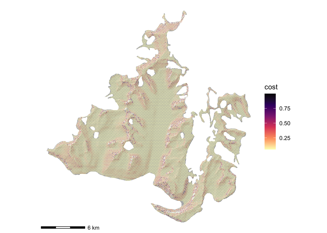
So let’s take a look… first, at a map of the network for reassurance - noting that since costs are different in each direction there’s no easy way to show this unambiguously. Some ‘holes’ in the network in steep areas are now apparent.

Code

hillshade_basemap +
  geom_sf(data = G |> get_graph_as_line_layer(), 
          aes(colour = cost), linewidth = 0.1) +
  scale_colour_viridis_c(option = "A", direction = -1) +
  theme_void()

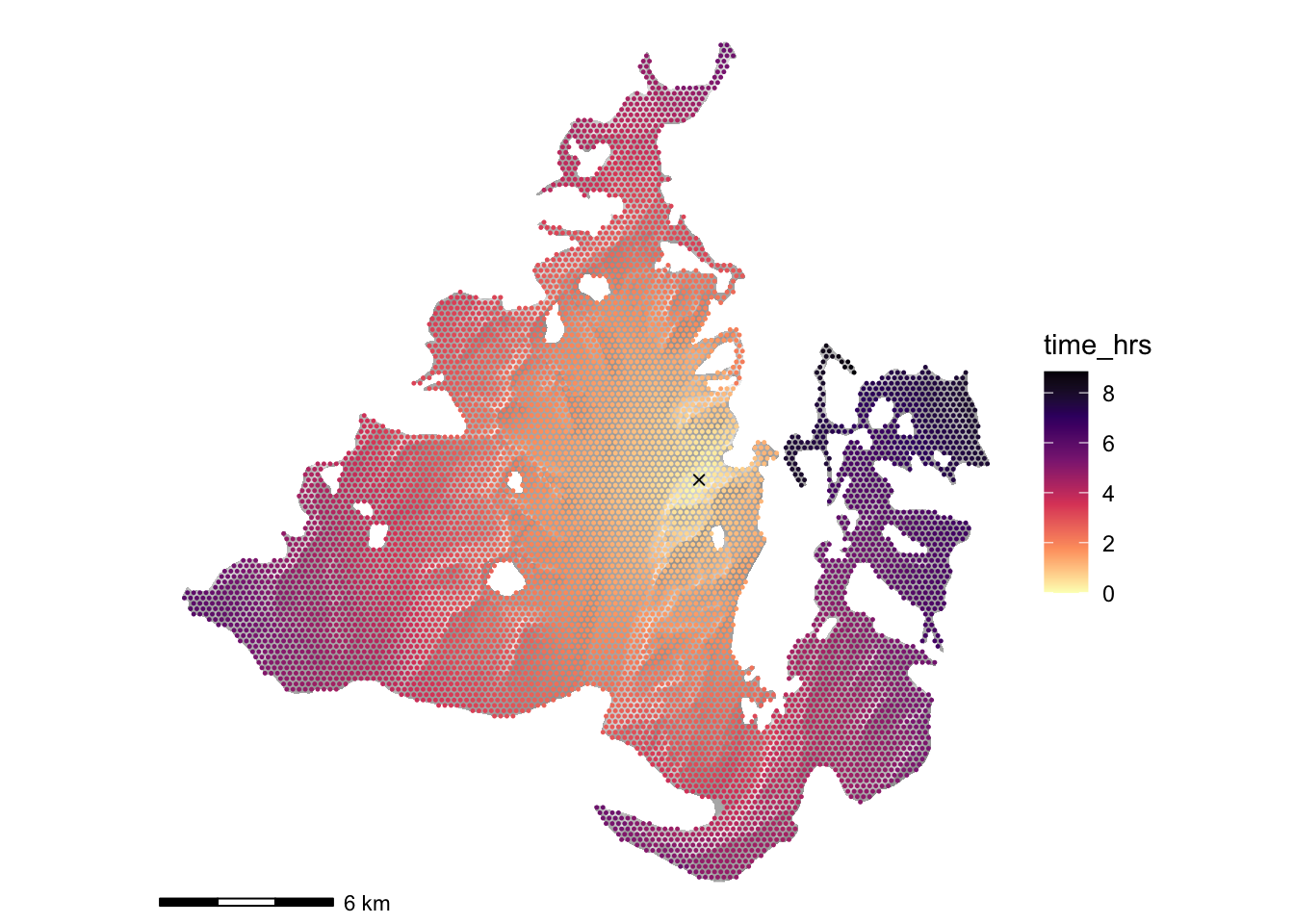
And just for assurance, here’s an estimated travel time map.

Code

# pick a random point as origin point for some examples
origin_i <- sample(seq_along(pts$geom), 1)[1]
origin <- c(pts$x[origin_i], pts$y[origin_i])

V(G)$time_hrs <- distances(G, v = c(V(G)[origin_i]), 
                           weights = edge_attr(G, "cost")) |> t()
df <- vertex.attributes(G) |> as.data.frame()

hillshade_basemap +
  geom_point(data = df, aes(x = x, y = y, colour = time_hrs), size = 0.2) +
  scale_colour_viridis_c(option = "A", direction = -1) +
  annotate("point", x = origin[1], y = origin[2], pch = 4) +
  coord_equal()