Refining hiking functions

Revisiting hiking function estimation with more data

Update History

Date	Changes
2024-09-26	Added an executive summary.
2024-09-23	Finalised the hiking function for use.
2024-09-19	Detailed the commentary.
2024-09-16	Initial post.

TL;DR Executive summary

The key findings are:

• GPS data must be filtered to support estimation of reasonable hiking functions. In particular: stopping locations (base camp, experimental sites, rest stops) must be filtered out. This filtering is performed by counting fixes in hexbins at 100m spacing and removing any fixes that fall in dense areas (50 fixes per bin was arbitrarily chosen after some experimentation). An alternative might be to obtain detailed information about the base camp and experimental sites for this season’s fieldwork.
• Also removed: observations associated with a slope estimate slope_h == 0. There are an anomalously large number of these and they depress estimated hiking speeds on the flat. Exploration of the data turned up no obvious reason for the existence of these fixes, so the pragmatic decision was taken to remove them. Many slope estimates close to 0 are present in the data in any case.
• Also removed: high turn angles (≥150°) and low reported GPS distances (≤2.5m) as these are both suggestive of ‘loitering’ not purposive movement.
• Hiking function estimation is readily carried out based on the complete remaining dataset. This seems preferable to an earlier approach using a smoothed version of the data derived from median speeds at a series of slope intervals. We have many data points, let’s use them!
• A Gaussian functional form seems to fit the data best.
• The differences between the hiking function derived for moraine and rock surfaces are plausible enough and strong enough to retain both functions and apply them separately to the setup of the hiking network.
• There are differences between individuals but since the purpose of this research is to estimate collective impacts across populations of scientists, there is no obvious way to incorporate such differences into the project.

library(here)
library(sf)
library(ggplot2)
library(hrbrthemes)
library(ggnewscale)
library(ggspatial)
library(minpack.lm)
library(dplyr)
library(tidyr)
library(stringr)

Organise the data

Now read the GPS data and associate with it different geology types. Contrary to the more detailed geology types shown in this notebook we use a column from the geology layer that distinguishes only moraine, rock, and ice. More detail than this is not readily validated, and also the GPS data available only crosses 8 of the 13 geology classes in the more detailed classification—and hence cannot be used to parameterise the more detailed classification anyway.

# gps data and its bbox
gps_data <- st_read(str_glue("{here()}/_data/cleaned-gps-data/all-gps-traces.gpkg"))
bb <- gps_data |> st_bbox() # this is to allow plotting restricted to GPS extents

# geologies data
geologies <- 
  st_read(str_glue("{here()}/_data/ata-scar-geomap-geology-v2022-08-clipped.gpkg")) |> 
  dplyr::select(POLYGTYPE) |>
  st_filter(bb |> st_as_sfc()) |> 
  mutate(cover = factor(POLYGTYPE))

# join geologies to the gps data
gps_geol <- gps_data |>
  mutate(slope_h2 = dh / dxyh) |>
  st_join(geologies) |>
  dplyr::select(-POLYGTYPE) |> 
  # we do not further consider (in this notebook) 'ice' terrain, nor
  # observations at negative elevations(!)
  filter(cover != "ice", height_m > 0) |>
  mutate(slope_h_round = round(slope_h * 10) / 10) |>
  drop_na()

Suppressing observations with slope_h == 0

One anomaly remains in the GPS data, which is hard to explain, but affects the estimation of models as carried out in the remainder of this notebook, namely a large number of observations with estimated slope_h of 0. This is apparent in a scatterplot of the data

ggplot(gps_geol) +
  geom_point(aes(x = slope_h, y = speed_km_h), size = 0.1, alpha = 0.1, pch = 19) +
  theme_ipsum_rc()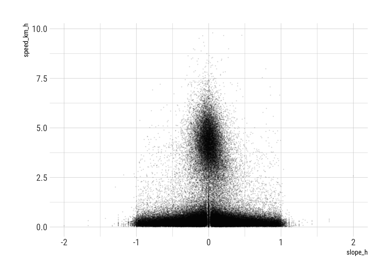

Even a cursory examination of a local smoothing of the speed of movement relative to slope demonstrates the effect of these observations on any estimation of rates of movement.

ggplot(gps_geol) +
  geom_boxplot(aes(x = round(slope_h, 1), y = speed_km_h, group = round(slope_h, 1)), 
               outlier.size = 0.2, colour = "grey", linewidth = 0.5) +
  stat_smooth(aes(x = slope_h, y = speed_km_h)) +
  theme_ipsum_rc()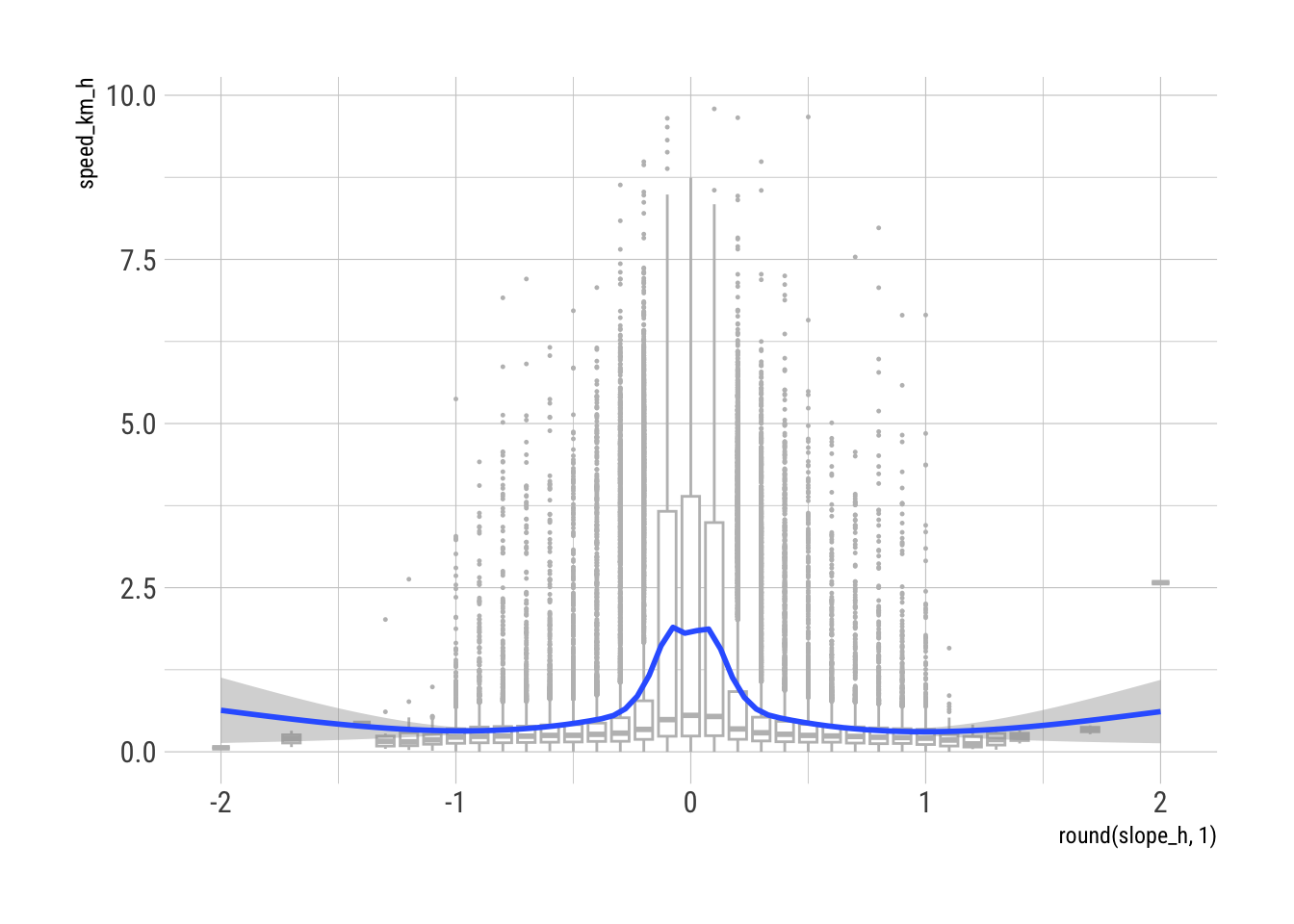

This concentration of observations at a single value seems likely to be an artifact of data collection, and so we avoid further difficulties by removing such observations as one part of the filtering discussed in the next section.

Filter out areas of non-purposive movement

Estimating a hiking function depends in part on only fitting functions to data recorded when subjects were purposefully moving.

One option is to filter on the density of GPS fixes - there are necessarily many more GPS fixes in and around the base camp than elsewhere. We can use hex binning to estimate density of fixes.

hexes <- gps_geol |> 
  st_make_grid(cellsize = 100, square = FALSE, what = "polygons") |>
  st_as_sf(crs = st_crs(gps_geol)) |>
  rename(geom = x) |>
  st_join(gps_geol |> mutate(id = row_number()), left = FALSE) |>
  group_by(geom) |>
  summarise(n = n(), n_persons = n_distinct(name)) |>
  ungroup()

We use this in conjunction with some other characteristics of the traces to filter data to fixes most likely to be associated with periods of purposive movement. Choice of cutoff values is fairly arbitrary. Experimentation with settings shows that exact values don’t matter greatly, the important thing is to exclude data in or around base camp, experimental sites, rests stops, etc. In any case, doing so (as shown in the plot which follows below, makes it difficult to argue for a meaningful difference in estimated hiking speeds vs. slope on the different geologies available in the GPS data).

gps_geol_purposive <- gps_geol |> 
  # see above
  filter(slope_h != 0) |>
  # these two remove 'dithering'
  filter(turn_angle < 150) |>
  filter(distance_m > 2.5) |>
  # remove fixes in densely trafficked areas
  st_join(hexes) |>
    filter(n <= 50)

A map to show the effect.

ggplot() +
  geom_sf(data = geologies, aes(fill = cover), linewidth = 0.1, colour = "white") +
  scale_fill_brewer(palette = "Pastel2") +
  new_scale_fill() +
  geom_sf(data = hexes |> filter(n <= 200), aes(fill = n), linewidth = 0) +
  scale_fill_viridis_c(option = "A", direction = 1) +
  geom_sf(data = gps_geol_purposive, size = 0.005, pch = 19, colour = "white") +
  coord_sf(xlim = bb[c(1, 3)], ylim = bb[c(2, 4)]) +
  annotation_scale(height = unit(0.1, "cm")) +
  theme_ipsum_rc()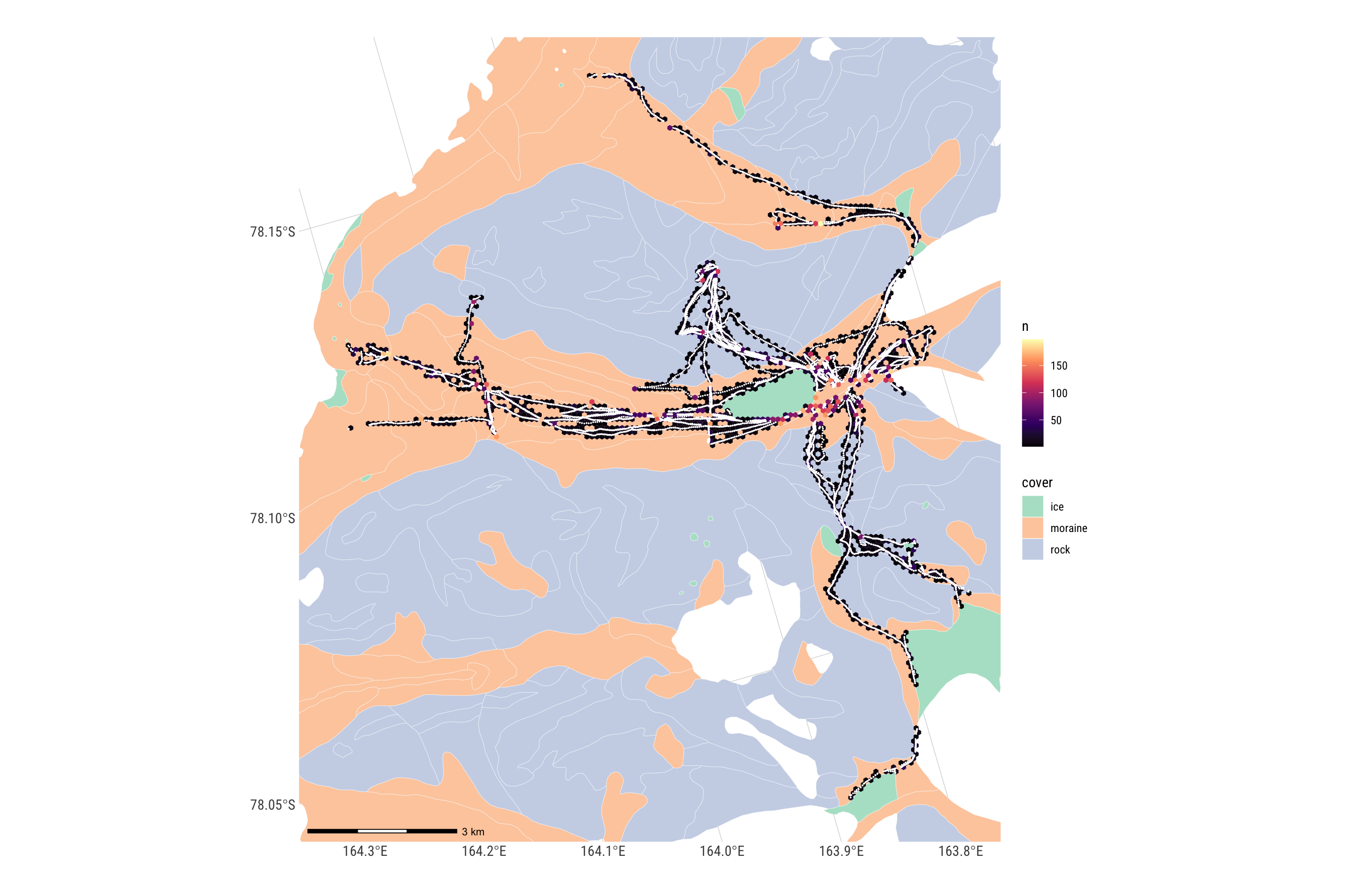

Estimate models

Functions to estimate models

get_gaussian_hiking_function <- function(df, percentile = 0.5) {
  nlsLM(speed_km_h ~ a * dnorm(slope_h, m, s), data = df,
        start = c(a = 5, m = 0, s = 0.5))
}

get_tobler_hiking_function <- function(df, percentile = 0.5) {
  nlsLM(speed_km_h ~ a * exp(-b * abs(slope_h + c)), data = df,
        start = c(a = 5, b = 3, c = 0.05))  
}

get_students_hiking_function <- function(df, percentile = 0.5) {
  nlsLM(speed_km_h ~ a * dt((slope_h + m), d), data = df,
                   start = c(a = 5, m = 0, d = 0.001))  
}

It is also convenient to have a function that returns estimated speeds as a slope-speed dataframe.

# makes a prediction data frame with x, y values
# slopes is a DF with one column called slope_h
get_model_prediction_df <- function(m, slopes) {
  data.frame(x = slopes, y = predict(m, data.frame(slope_h = slopes$slope_h)))
}

Now estimate hiking functions split by geology.

slopes <- data.frame(slope_h = -150:150 / 100)

hiking_functions <- list(
  gaussian = get_gaussian_hiking_function,
  tobler = get_tobler_hiking_function,
  students = get_students_hiking_function
)
covers <- c("moraine", "rock")

pc <- 0.5
nbins <- 10

models <- list()
predictions <- list()
inputs <- list()
i <- 1
for (name in names(hiking_functions)) {
  for (cover_type in covers) {
    df <- gps_geol_purposive |> 
      filter(cover == cover_type) 
    # |>
    #   get_percentile_summary(percentile = pc, num_bins = nbins)
    m <- hiking_functions[[name]](df, pc)
    models[[cover_type]][[name]] <- m
    predictions[[i]] <- get_model_prediction_df(m, slopes) |>
      mutate(cover = cover_type, model = name)
    inputs[[i]] <- df |>
      mutate(cover = cover_type, model = name)
    i <- i + 1
  }
}
model_predictions <- bind_rows(predictions)
input_data <- bind_rows(inputs)

Inspection of initial models

ggplot() +
  geom_boxplot(data = gps_geol_purposive,
               aes(x = slope_h_round, y = speed_km_h, group = slope_h_round),
               outlier.size = 0.35, colour = "grey", linewidth = 0.5) +
  # geom_point(data = input_data, aes(x = slope_h, y = speed_km_h)) + 
  geom_line(data = model_predictions, aes(x = slope_h, y = y, colour = model)) +
  xlab("Slope") + ylab("Speed, km/h") +
  facet_wrap( ~ cover, ncol = 3) +
  theme_ipsum_rc()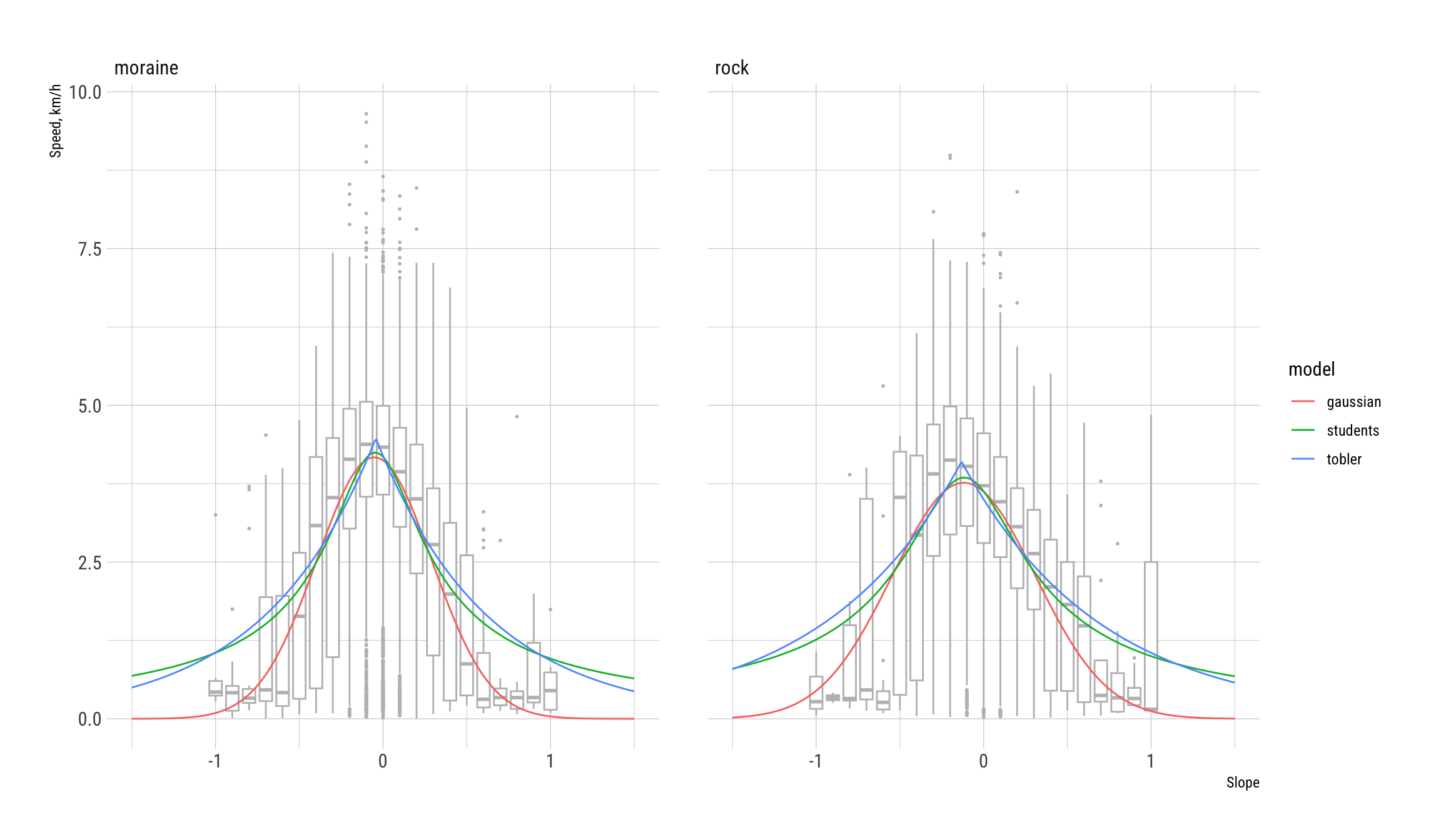

Based on these results (and also some prior exploration):

• Although models can be estimated for ‘ice’ we consider ice impassable, as it is clear from mapping the GPS data that any supposed movement across ‘ice’ is due to inaccuracies in the data. Hence this geology cover has been removed from consideration.
• It appears that the top speed attainable across ‘moraine’ is slightly higher than on ‘rock’, which seems reasonable.
• It may be that the speed attained across ‘moraine’ falls away more rapidly with slope than on ‘rock’. This is not implausible: ‘moraine’ terrain might be slippy and somewhat treacherous to cross on steeper slopes.

The Gaussian functional forms of the hiking function have the best ‘fit’ based on the residual sum of squares statistic (and AIC and log-likelihood).

Are the hiking functions on the two terrains different enough to use both?

But should we use different models for the two surface covers? The differences above are not substantial. We can explore their overlap by Monte-Carlo simulation of the fitted models. This unfortunately is not something models generated by minpack.lm::nlsLM can do using the base R predict.nls functions. The following function, obtained from this post has been used for this purpose and appears to work satisfactorily.

predictNLS <- function(object, newdata, level = 0.95, nsim = 10000, ...) {
  require(MASS, quietly = TRUE)
  ## get right-hand side of formula
  RHS <- as.list(object$call$formula)[[3]]
  EXPR <- as.expression(RHS)
  ## all variables in model
  VARS <- all.vars(EXPR)
  ## coefficients
  COEF <- coef(object)
  ## extract predictor variable    
  predNAME <- setdiff(VARS, names(COEF))  
  ## take fitted values, if 'newdata' is missing
  if (missing(newdata)) {
    newdata <- eval(object$data)[predNAME]
    colnames(newdata) <- predNAME
  }
  ## check that 'newdata' has same name as predVAR
  if (names(newdata)[1] != predNAME) stop("newdata should have name '", predNAME, "'!")
  ## get parameter coefficients
  COEF <- coef(object)
  ## get variance-covariance matrix
  VCOV <- vcov(object)
  ## augment variance-covariance matrix for 'mvrnorm' 
  ## by adding a column/row for 'error in x'
  NCOL <- ncol(VCOV)
  ADD1 <- c(rep(0, NCOL))
  ADD1 <- matrix(ADD1, ncol = 1)
  colnames(ADD1) <- predNAME
  VCOV <- cbind(VCOV, ADD1)
  ADD2 <- c(rep(0, NCOL + 1))
  ADD2 <- matrix(ADD2, nrow = 1)
  rownames(ADD2) <- predNAME
  VCOV <- rbind(VCOV, ADD2) 
  ## iterate over all entries in 'newdata' as in usual 'predict.' functions
  NR <- nrow(newdata)
  respVEC <- numeric(NR)
  seVEC <- numeric(NR)
  varPLACE <- ncol(VCOV)   
  ## define counter function
  counter <- function (i) {
    if (i%%10 == 0) 
      cat(i)
    else cat(".")
    if (i%%50 == 0) 
      cat("\n")
    flush.console()
  }
  outMAT <- NULL 
  for (i in 1:NR) {
    counter(i)
    ## get predictor values and optional errors
    predVAL <- newdata[i, 1]
    if (ncol(newdata) == 2) predERROR <- newdata[i, 2] else predERROR <- 0
    names(predVAL) <- predNAME  
    names(predERROR) <- predNAME  
    ## create mean vector for 'mvrnorm'
    MU <- c(COEF, predVAL)
    ## create variance-covariance matrix for 'mvrnorm'
    ## by putting error^2 in lower-right position of VCOV
    newVCOV <- VCOV
    newVCOV[varPLACE, varPLACE] <- predERROR^2
    ## create MC simulation matrix
    simMAT <- mvrnorm(n = nsim, mu = MU, Sigma = newVCOV, empirical = TRUE)
    ## evaluate expression on rows of simMAT
    EVAL <- try(eval(EXPR, envir = as.data.frame(simMAT)), silent = TRUE)
    if (inherits(EVAL, "try-error")) stop("There was an error evaluating the simulations!")
    ## collect statistics
    PRED <- data.frame(predVAL)
    colnames(PRED) <- predNAME   
    FITTED <- predict(object, newdata = data.frame(PRED))
    MEAN.sim <- mean(EVAL, na.rm = TRUE)
    SD.sim <- sd(EVAL, na.rm = TRUE)
    MEDIAN.sim <- median(EVAL, na.rm = TRUE)
    MAD.sim <- mad(EVAL, na.rm = TRUE)
    QUANT <- quantile(EVAL, c((1 - level)/2, level + (1 - level)/2))
    RES <- c(FITTED, MEAN.sim, SD.sim, MEDIAN.sim, MAD.sim, QUANT[1], QUANT[2])
    outMAT <- rbind(outMAT, RES)
  }
  colnames(outMAT) <- c("fit", "mean", "sd", "median", "mad", names(QUANT[1]), names(QUANT[2]))
  rownames(outMAT) <- NULL
  cat("\n")
  return(outMAT)  
}

Before applying this, we also estimate a model from all the data

df <- gps_geol_purposive 
m3 <- get_gaussian_hiking_function(df, pc)
models[["all"]][["gaussian"]] <- m
model_predictions <- model_predictions |>
  bind_rows(get_model_prediction_df(m, slopes) |> 
              mutate(cover = "all", model = "gaussian"))
input_data <- input_data |>
  bind_rows(df |> mutate(cover = "all", model = "gaussian"))

And now determine confidence intervals across all three models.

conf <- 0.95
pred1 <- predictNLS(models[["moraine"]][["gaussian"]], newdata = slopes, level = conf) |>
  as.data.frame() |>
  mutate(x = slopes$slope_h, cover = "moraine")

.........10.........20.........30.........40.........50
.........60.........70.........80.........90.........100
.........110.........120.........130.........140.........150
.........160.........170.........180.........190.........200
.........210.........220.........230.........240.........250
.........260.........270.........280.........290.........300
.

pred2 <- predictNLS(models[["rock"]][["gaussian"]], newdata = slopes, level = conf) |>
  as.data.frame() |>
  mutate(x = slopes$slope_h, cover = "rock")

.........10.........20.........30.........40.........50
.........60.........70.........80.........90.........100
.........110.........120.........130.........140.........150
.........160.........170.........180.........190.........200
.........210.........220.........230.........240.........250
.........260.........270.........280.........290.........300
.

pred3 <- predictNLS(m3, newdata = slopes, level = conf) |>
  as.data.frame() |>
  mutate(x = slopes$slope_h, cover = "all")

.........10.........20.........30.........40.........50
.........60.........70.........80.........90.........100
.........110.........120.........130.........140.........150
.........160.........170.........180.........190.........200
.........210.........220.........230.........240.........250
.........260.........270.........280.........290.........300
.

predictions <- bind_rows(pred1, pred2, pred3)

And now we can overplot the models showing their 95% confidence intervals.

ggplot() +
  geom_ribbon(data = predictions |> filter(cover != "all"), 
              aes(x = x, ymin = `2.5%`, ymax = `97.5%`, group = cover, fill = cover), 
              alpha = 0.35, linewidth = 0) + 
  scale_fill_brewer(palette = "Set1", name = "Terrain") +
  geom_ribbon(data = predictions |> filter(cover == "all"), 
              aes(x = x, ymin = `2.5%`, ymax = `97.5%`), 
              colour = "black", lty = "dashed", fill = "#00000000", linewidth = 0.35) +
  geom_line(data = predictions |> filter(cover == "all"), aes(x = x, y = mean)) +
  xlab("Slope") + ylab("Speed, km/h") +
  theme_ipsum_rc()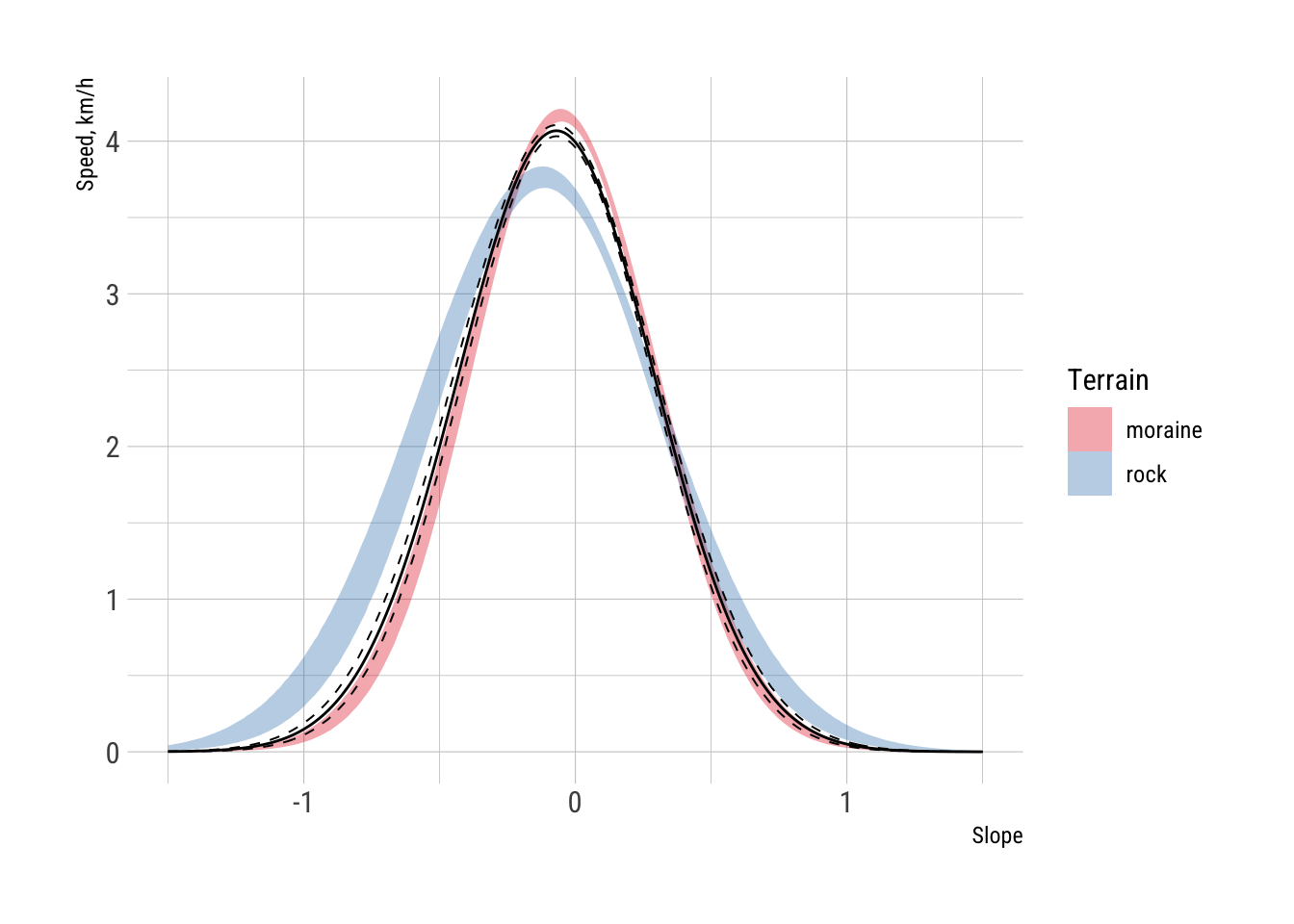

There is a clear difference between the moraine and rock estimates, both in the maximum speeds attained, and interestingly (and convincingly) in the slope at which this maximum speed is attained. Both terrains admit faster movement downhill, but a steeper downhill is where the fastest speed is attainable on rocky surfaces, and in fact downhill movement on rocky surfaces is faster at most slope angles. Uphill movement is similar on both terrain types. This makes sense when we consider that moraines consist of loose gravels which can be treacherous especially when moving downhill. The ‘all’ terrain model (black lines) matches quite closely the moraine model, but is a poor fit to the rocky terrain model.

Two estimated hiking functions

The two functions we are left with are

ggplot() + 
  geom_boxplot(data = gps_geol_purposive,
               aes(x = slope_h_round, y = speed_km_h, group = slope_h_round),
               outlier.size = 0.35, colour = "grey", linewidth = 0.5) +
  geom_ribbon(data = predictions |> filter(cover != "all"), 
            aes(x = x, ymin = `2.5%`, ymax = `97.5%`, fill = cover), alpha = 0.35) +
  scale_fill_brewer(palette = "Set1", name = "Terrain") +
  geom_line(data = predictions |> filter(cover != "all"), 
            aes(x = x, y = mean, colour = cover), linewidth = 0.75) +
  scale_colour_brewer(palette = "Set1", name = "Terrain") +
  theme_ipsum_rc()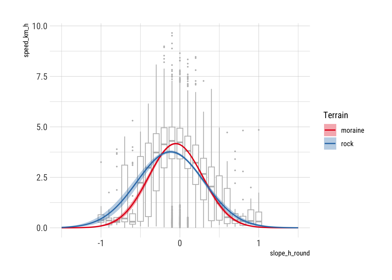

The equations for these function given the model summaries below

models[["moraine"]][["gaussian"]]

Nonlinear regression model
  model: speed_km_h ~ a * dnorm(slope_h, m, s)
   data: df
       a        m        s 
 3.59025 -0.05259  0.34348 
 residual sum-of-squares: 17728

Number of iterations to convergence: 5 
Achieved convergence tolerance: 1.49e-08

models[["rock"]][["gaussian"]]

Nonlinear regression model
  model: speed_km_h ~ a * dnorm(slope_h, m, s)
   data: df
      a       m       s 
 4.0302 -0.1188  0.4272 
 residual sum-of-squares: 8050

Number of iterations to convergence: 5 
Achieved convergence tolerance: 1.49e-08

noting that the Gaussian form is \(\frac{1}{\sqrt{2\pi\sigma^2}}e^{-\frac{(x-\mu)^2}{2\sigma^2}}\), calculating out all the constants, are given by

\[ \begin{eqnarray} v_{\mathrm{moraine}} & = & 4.166092\,e^{-\frac{(s+0.05259)^2}{0.2363969}} \\ v_{\mathrm{rock}} & = & 3.763617\,e^{-\frac{(s+0.1188)^2}{0.3649997}} \end{eqnarray} \]

And here is a function implementing this

est_hiking_function <- function(slope, terrain = "moraine") {
  if (terrain == "moraine") {
    4.166092 * exp(-(slope + 0.05259) ^ 2 / 0.2363969)
  } else {
    3.763617 * exp(-(slope + 0.1188) ^ 2 / 0.3649997)
  }
}

Overall, it is unlikely that these details will much affect overall outcomes of the analysis, although it seems worth making the most of the available data, which this approach will do.

The most impactful aspect of changes in the top speed of the hiking function will be on the choice of ‘cutoff’ cost for the betweenness measures. However, this choice is subjective and indicative only, so it is difficult to develop any systematic rules around calibration of the hiking function, or the choice of betweenness cutoff cost.

Addendum: what about variation between hikers

While there are differences between hikers (as shown below), since the purpose of this work is to determine a mean impact on the land aggregated over many different hikers, there seems no sensible way to include this information in the hiking function applied.

For simplicity here, we form estimates based on all the data not differentiated by terrain.

names <- gps_geol_purposive$name |> unique()
models <- list()
results <- list()
i <- 1
for (the_name in names) {
  df <- gps_geol_purposive |> 
    filter(name == the_name)
  m <- df |> get_gaussian_hiking_function(percentile = pc)
  models[[the_name]] <- m
  results[[i]] <- m |> 
    get_model_prediction_df(slopes) |>
    mutate(name = the_name)
  i <- i + 1
}
model_predictions <- results |> 
  bind_rows()

ggplot() +
  geom_boxplot(data = gps_geol_purposive,
               aes(x = slope_h_round, y = speed_km_h, group = slope_h_round),
               outlier.size = 0.25, colour = "darkgrey") +
  geom_line(data = model_predictions, aes(x = slope_h, y = y)) +
  xlab("Slope") + ylab("Speed, km/h") +
  facet_wrap( ~ name) +
  theme_ipsum_rc()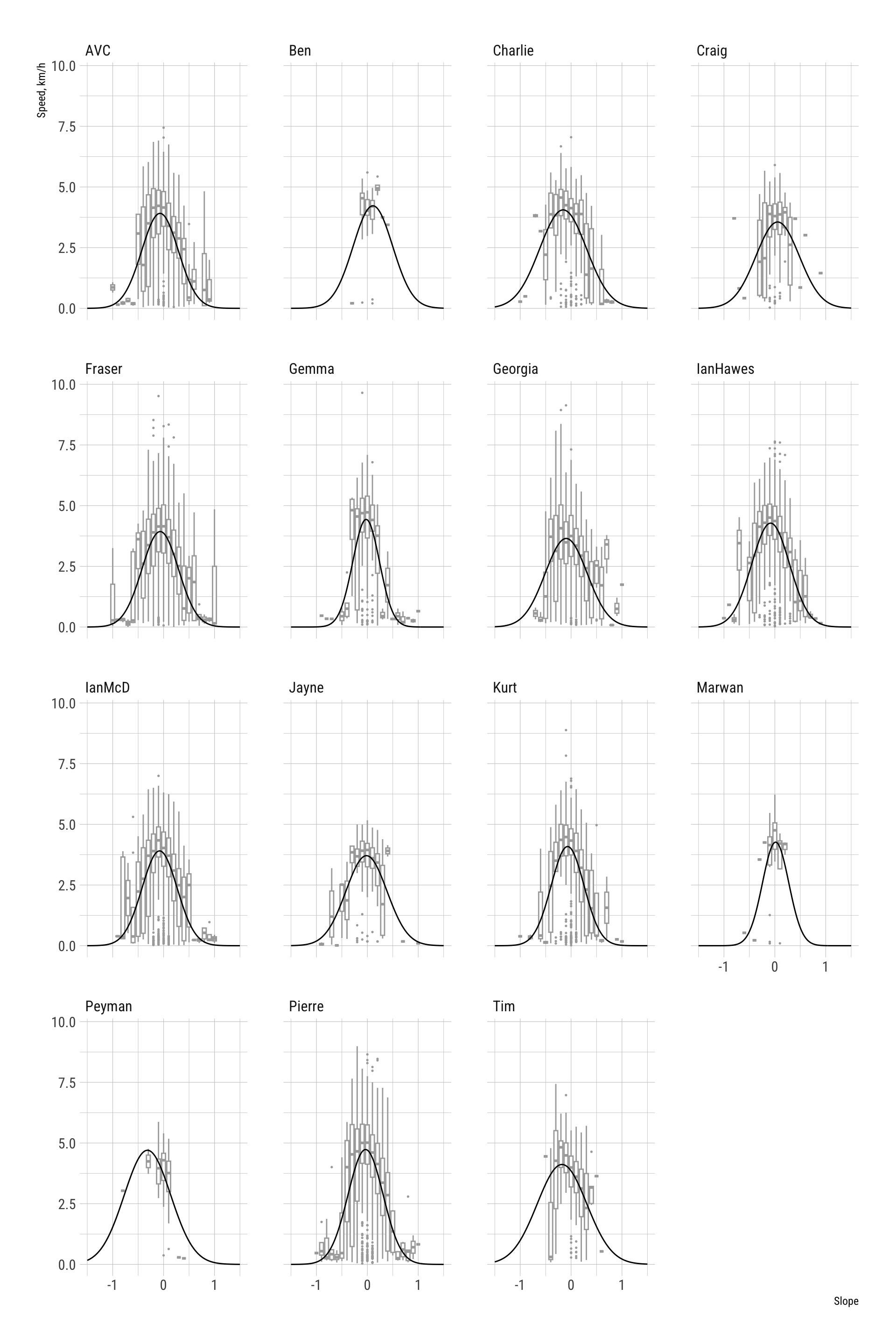

SUPERSEDED

Smoothed speed-slope profiles

In earlier work, hiking function estimation was based on median speeds at a small number of slope intervals. This appears to be unnecessary but code is included below for completeness.

It is helpful to instead summarise the data at some chosen percentile of the distribution of recorded speeds within in slope interval bins. The following function does this and the result is illustrated.

# helper function to reduce data to a more smoothed form
get_percentile_summary <- function(df, percentile, num_bins) {
  df |> mutate(slope_bin = cut_interval(slope_h, num_bins)) |>
    group_by(slope_bin) |>
    summarise(
      slope_h = mean(slope_h),
      speed_km_h = quantile(speed_km_h, percentile),
      percentile = percentile) |>
    ungroup()
}

We can plot these to get a feel for what might be a sensible percentile to apply.

summary_speed_by_slope_df <- (1:19 / 20) |>
  as.list() |>
  lapply(get_percentile_summary, df = gps_geol_purposive, num_bins = 10) |>
  bind_rows()

ggplot() +
  geom_point(data = gps_geol_purposive, aes(x = slope_h, y = speed_km_h), colour = "black", size = 0.25, alpha = 0.1) +
  geom_line(data = summary_speed_by_slope_df, aes(x = slope_h, y = speed_km_h, colour = percentile, group = percentile)) +
  scale_colour_distiller(palette = "Spectral") +
  theme_ipsum_rc()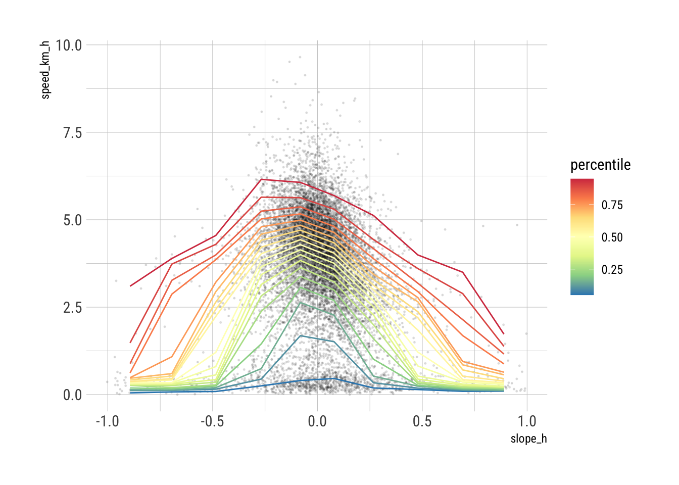

Based on this plot, the median (percentile = 0.5) choice seems the most reasonable, as it is less affected by occasional high outlier high speed movement.