Taking stock

Progress to 4 September, 2024

Author

David O’Sullivan

Published

September 4, 2024

Update History

Date	Changes
2024-09-26	Added some notes on future work.
2024-08-29	Initial post.

This notebook sets out progress to date (end of August 2024).

Since it was assembled, some refinements to the process have been developed:

Further refinement of hiking function estimation suggests that there is no need to include terrain factors in the cost calculation for network edges.
Hiking networks themselves should remove steep/slow edges. This became apparent in developing code for betweenness calculations based on a limited set of origins and destinations, when imposing a cost cutoff reveals the existence of some very costly edges in networks (this should have been apparent sooner… but so it goes).

Code

library(here)
library(stringr)
library(ggplot2)
library(ggnewscale)
library(whitebox)
library(ggpubr)
library(ggspatial)
library(tmap)

source(str_glue("{here()}/scripts/raster-to-graph-functions.R"))
base_folder <- here()
data_folder <- str_glue("{base_folder}/_data")
dem_folder  <- str_glue("{base_folder}/_data/dem")

Definition of the study area

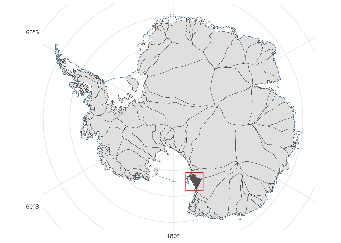
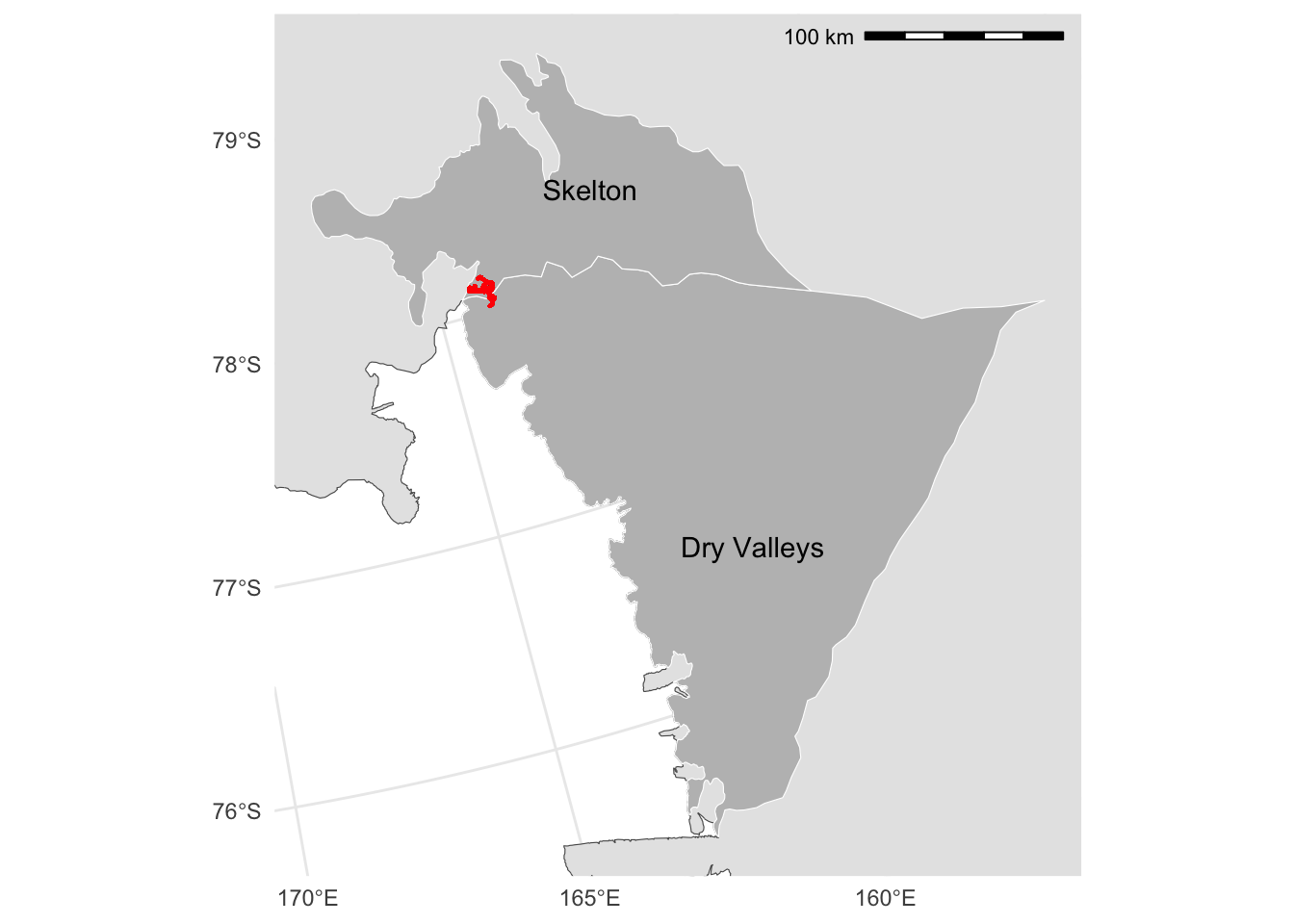
I’ve settled on two ‘basins’, Skelton and Dry Valleys, as defined by the NASA Making Earth System Data Records for Use in Research Environments (MEaSUREs) project, downloadable from here.¹

Code

coastline <- st_read(str_glue("{data_folder}/coastline.gpkg"))
basins <- st_read(str_glue("{dem_folder}/antarctic-basins.gpkg"))
study_basins <- st_read(str_glue("{dem_folder}/dry-valleys-and-skelton.gpkg"))
study_area <- st_read(str_glue("{dem_folder}/study-area-extent.gpkg"))
gps_data <- st_read(str_glue("{data_folder}/cleaned-gps-data/all-gps-traces.gpkg"))
tiles <- st_read(str_glue("{dem_folder}/REMA-index-included-tiles.gpkg"))
shade <- rast(str_glue("{dem_folder}/32m/dry-valleys-combined-32m-browse.tif"))
shade8 <- shade |>
  terra::aggregate(8) |>
  as.data.frame(xy = TRUE) |>
  rename(shade = `15_35_32m_v2.0_browse`)
geology <- st_read(str_glue("{data_folder}/ata-scar-geomap-geology-v2022-08-clipped.gpkg"))
contiguous_geologies <- st_read(str_glue("{data_folder}/dry-valleys/common-inputs/contiguous-geologies.gpkg"))

Code

bb <- st_bbox(study_area)
ggplot() +
  geom_sf(data = basins) + 
  geom_sf(data = coastline, colour = "#5588aa", fill = "#00000000") +
  geom_sf(data = study_area, fill = "#666666", colour = "white") +
  annotate("rect", xmin = bb[1], ymin = bb[2], xmax = bb[3], ymax = bb[4], fill = "#00000000", colour = "red") +
  theme_minimal()

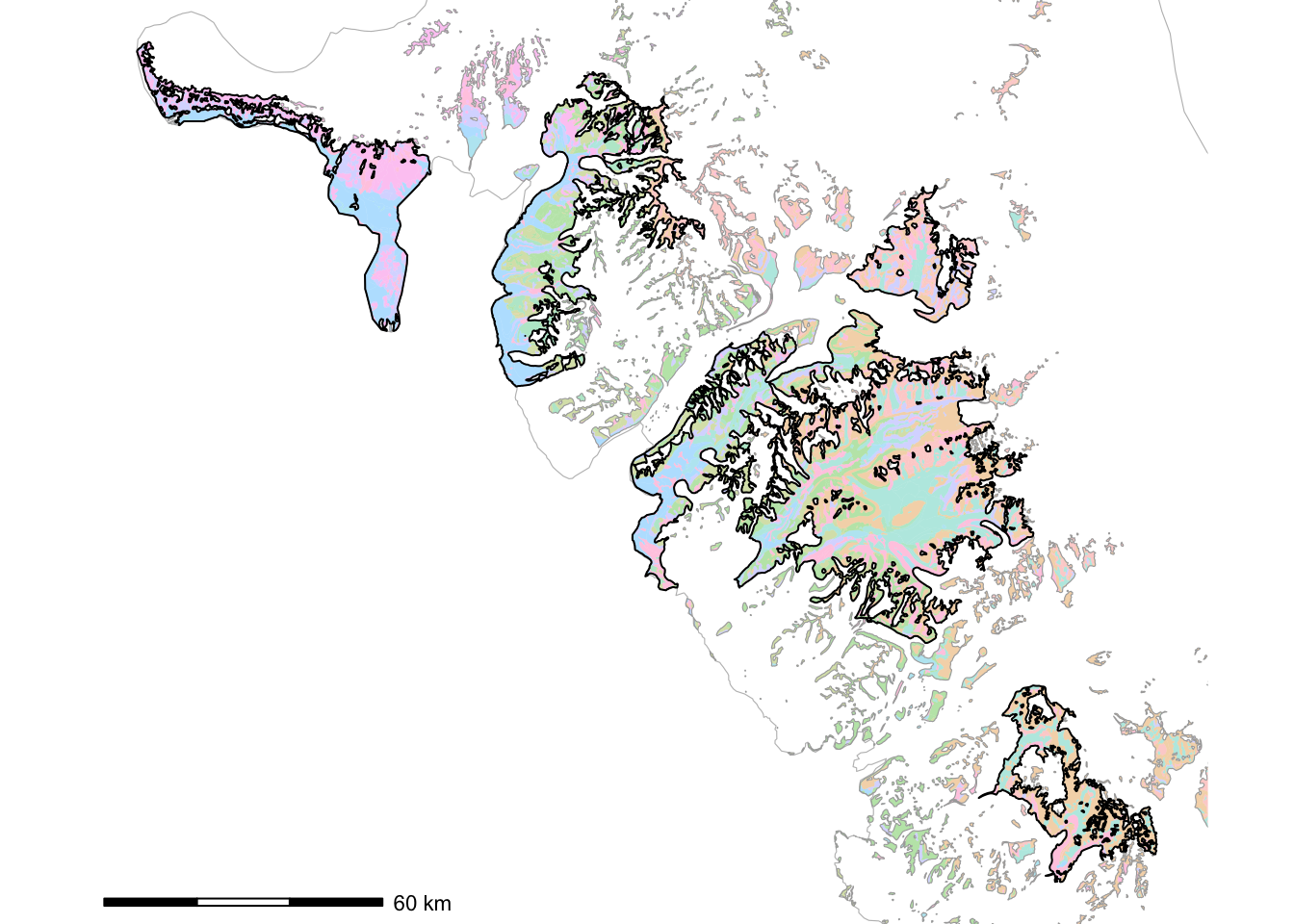
Looking more closely, Skelton was included in the study area extent because the provided GPS data from the 2015-16 season (shown in red below) extended into this basin in addition the Dry Valleys basin.

Code

ggplot() +
  geom_sf(data = coastline) +
  geom_sf(data = study_basins, fill = "grey", colour = "white") +
  geom_sf(data = gps_data, colour = "red", size = 0.025, title = "GPS data") +
  geom_sf_text(data = study_basins, aes(label = NAME)) +
  coord_sf(xlim = bb[c(1, 3)], ylim = bb[c(2, 4)]) +
  annotation_scale(height = unit(0.1, "cm"), location = "tr") +
  theme_minimal() +
  theme(axis.title = element_blank())

DEM data

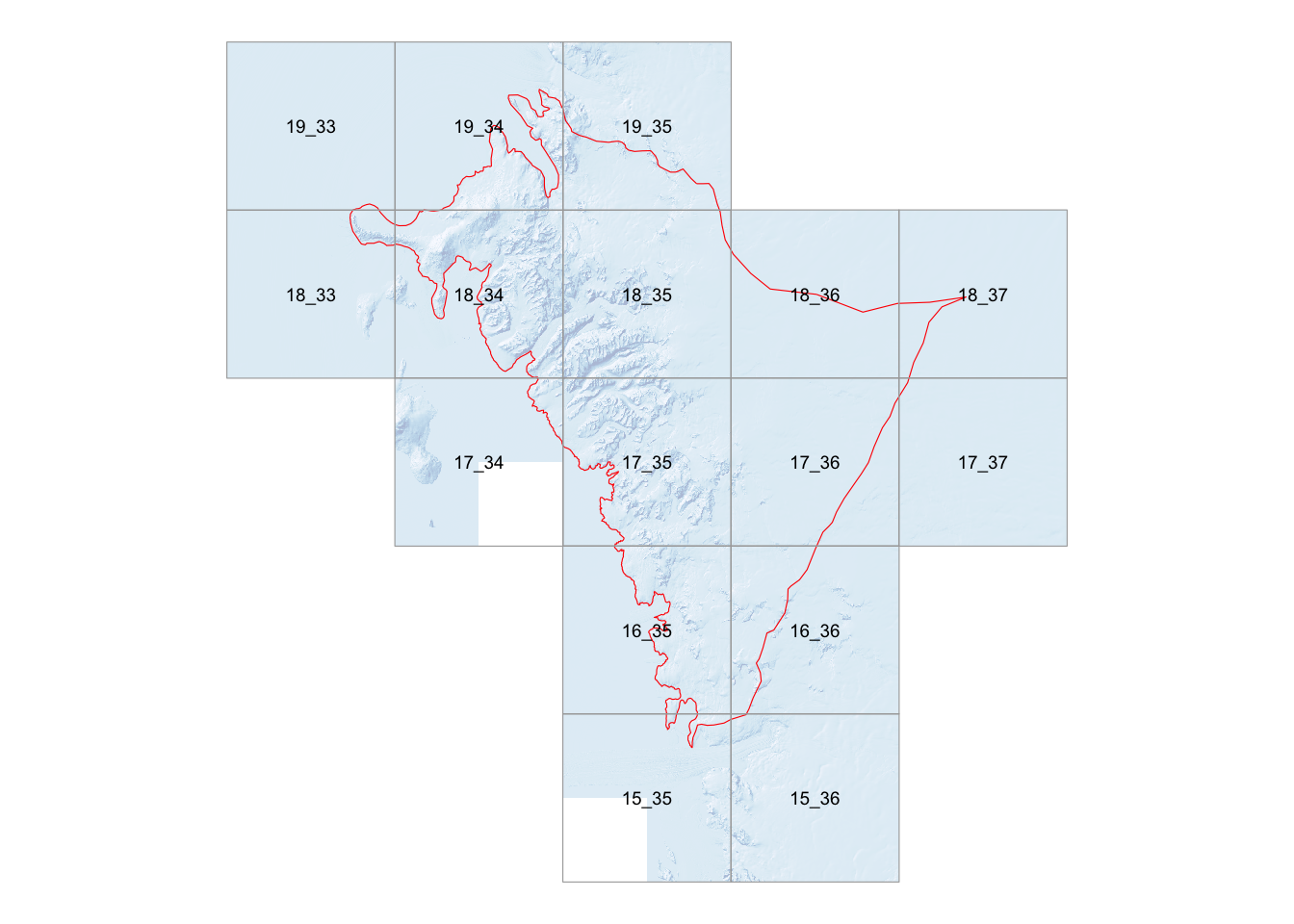
Based on this study area DEM data was assembled from the REMA project ² downloaded from ftp.data.pgc.umn.edu, using at least to begin the 32m resolution product, extending across tiles as shown below.

Code

ggplot() +
  geom_raster(data = shade8, aes(x = x, y = y, fill = shade), alpha = 0.35) +
  scale_fill_distiller(palette = "Blues", guide = "none") +
  geom_sf(data = study_area, fill = "#00000000", colour = "red") +
  geom_sf(data = tiles, fill = "#00000000", colour = "darkgrey") +
  geom_sf_text(data = tiles, aes(label = tile), size = 2.5) +
  theme_void()

Definition of areas of interest

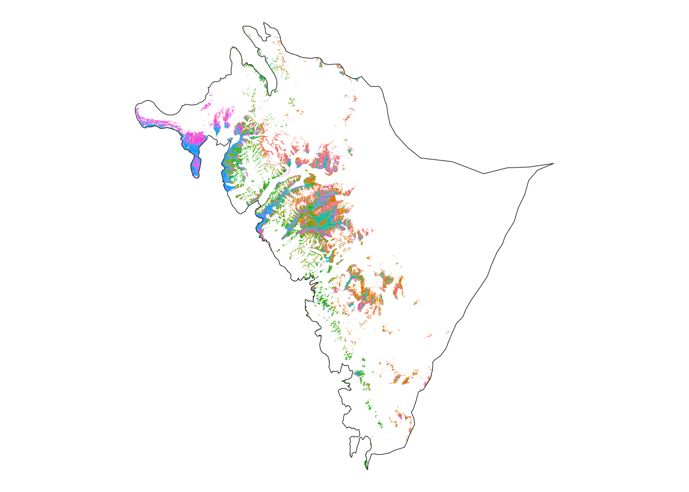
Much of the area delineated above is covered in permanent snow and ice. To delineate areas for closer study we use areas of classified geology obtained from the GNS GeoMAP ³ and downloaded from here

This layer is clipped to the study area extent. Colours in the map below are randomly signed and indicative only.

Code

ggplot() + 
  geom_sf(data = geology, aes(fill = SIMPDESC), linewidth = 0) +
  guides(fill = "none") +
  geom_sf(data = study_area, fill = "#00000000", colour = "black") +
  theme_void()

The geology layer serves two purposes:

Delineation of areas of interest: large regions of contiguous geology are chosen as study areas
Estimation of relative movement costs for building the hiking network

Areas of interest

The five largest regions of contiguous geology in the study area have been chosen for closer study. These range in extent from almost 2600 to around 320 sq.km.

Code

top5 <- contiguous_geologies |> arrange(desc(area)) |> slice(1:5)
bb <- st_bbox(top5)
ggplot() +
  geom_sf(data = study_area, fill = "#00000000", colour = "grey") +
  geom_sf(data = geology, aes(fill = SIMPDESC), linewidth = 0, alpha = 0.35) +
  geom_sf(data = contiguous_geologies, fill = "#00000000", colour = "darkgrey") +
  geom_sf(data = top5, fill = "#00000000", colour = "black", linewidth = 0.35) +
  coord_sf(xlim = bb[c(1, 3)], ylim = bb[c(2, 4)]) +
  guides(fill = "none") +
  annotation_scale(height = unit(0.1, "cm")) +
  theme_void()

Relative movement cost

For the time being a very crude relative movement rate classification assigning any geology including the term till a cost 1.5, any containing the term rock a cost 2, and all other areas (water and ice) a null value -999 has been used. Better choices might be 1.19 (or 1.67) for till and 2.5 for rock per values cited in the documentation of the R movecost package, as follows:

Cover	Cost
Blacktop roads, improved dirt paths, cement	1.00
Lawn grass	1.03
Loose beach sand	1.19
Disturbed ground (former stone quarry)	1.24
Horse riding path, flat trails and meadows	1.25
Tall grassland (with thistle and nettles)	1.35
Open space above the treeline (i.e., 2000 m asl)	1.50
Bad trails, stony outcrops and river beds	1.67
Off-paths	1.67
Bog	1.79
Off-path areas below the treeline (pastures, forests, heathland)	2.00
Rock	2.50
Swamp, water course	5.00

These choices remain open for discussion and adjustment, in combination with determination of localised hiking functions from the provided GPS data.

Current results: an example

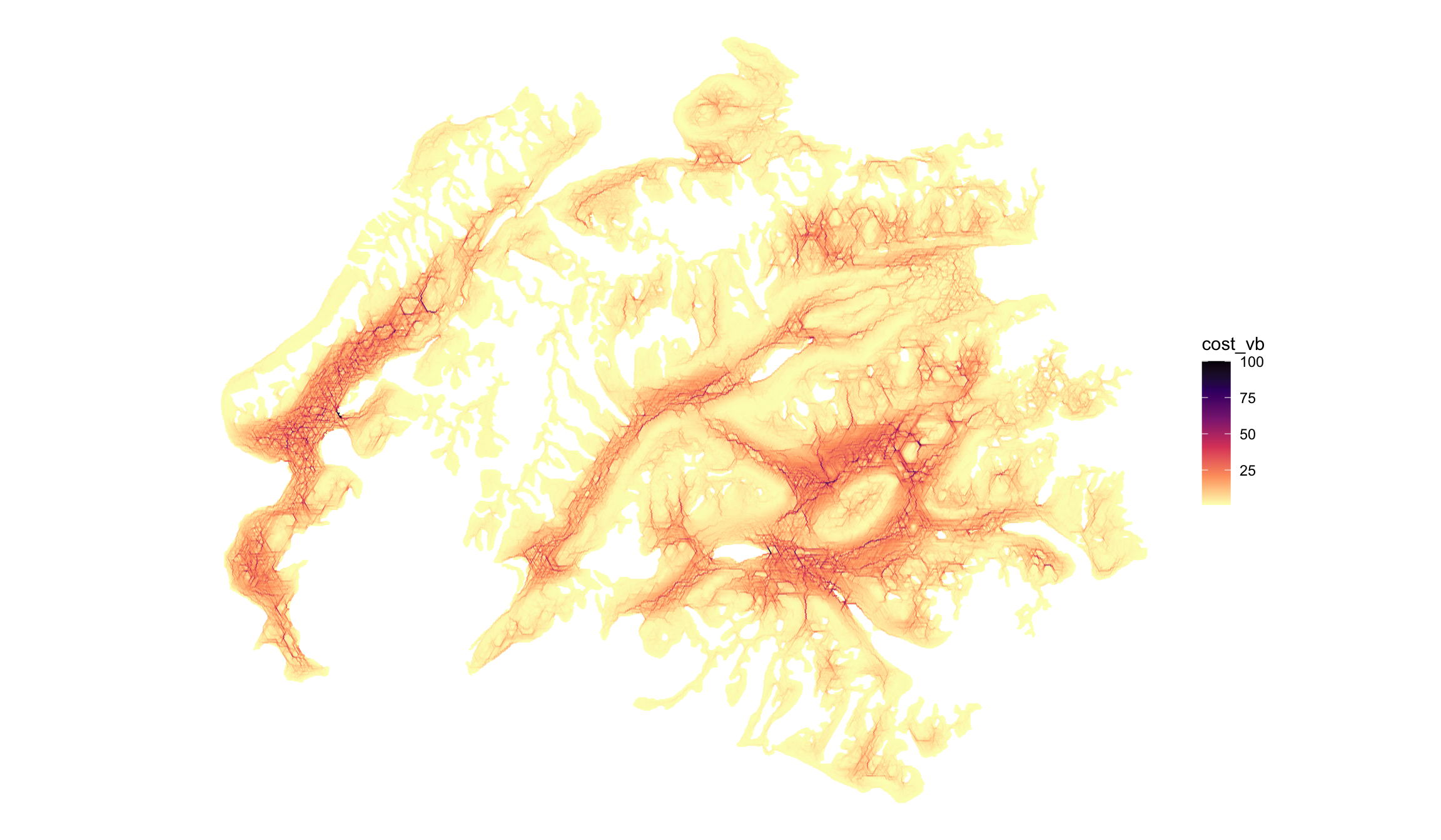
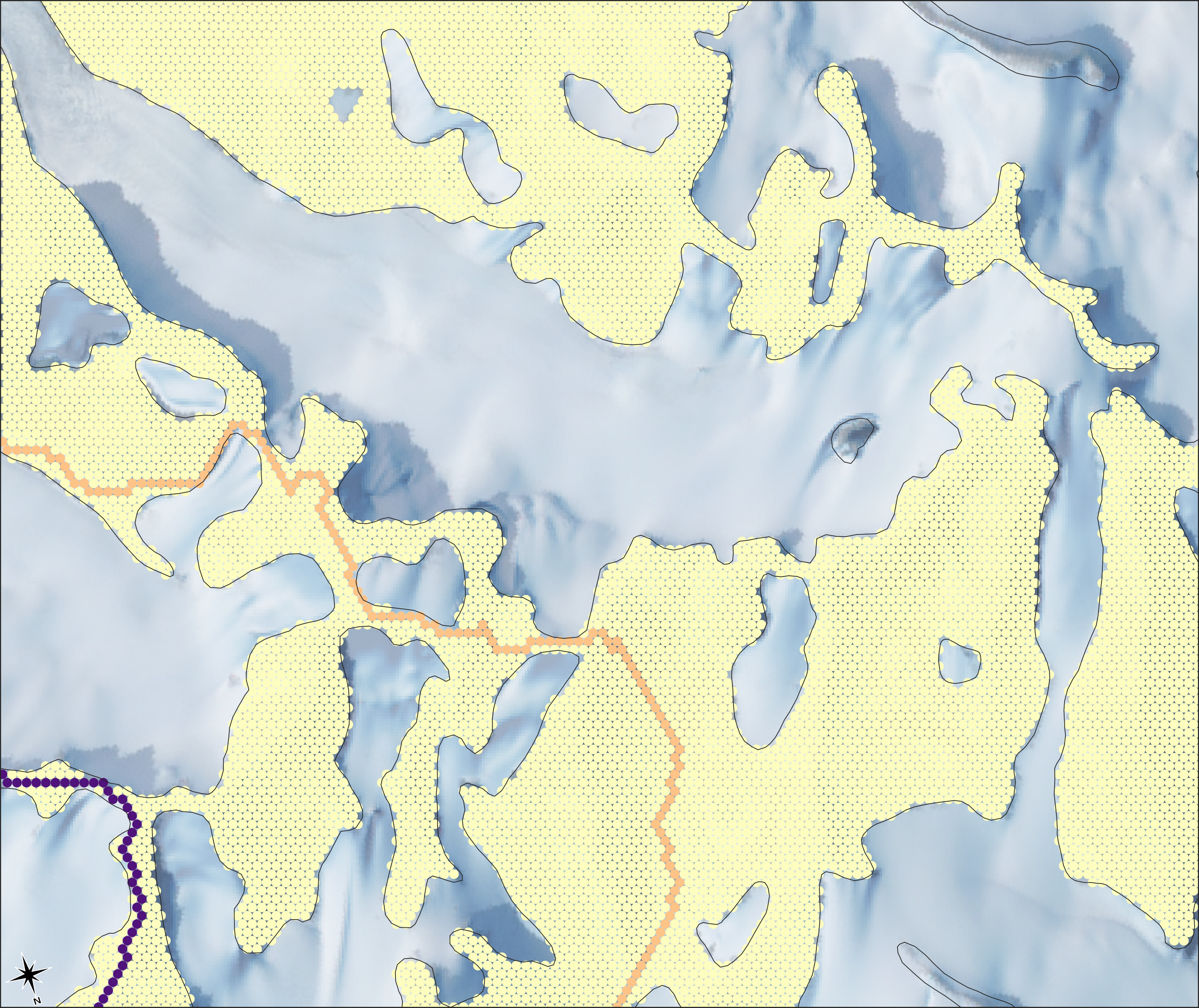
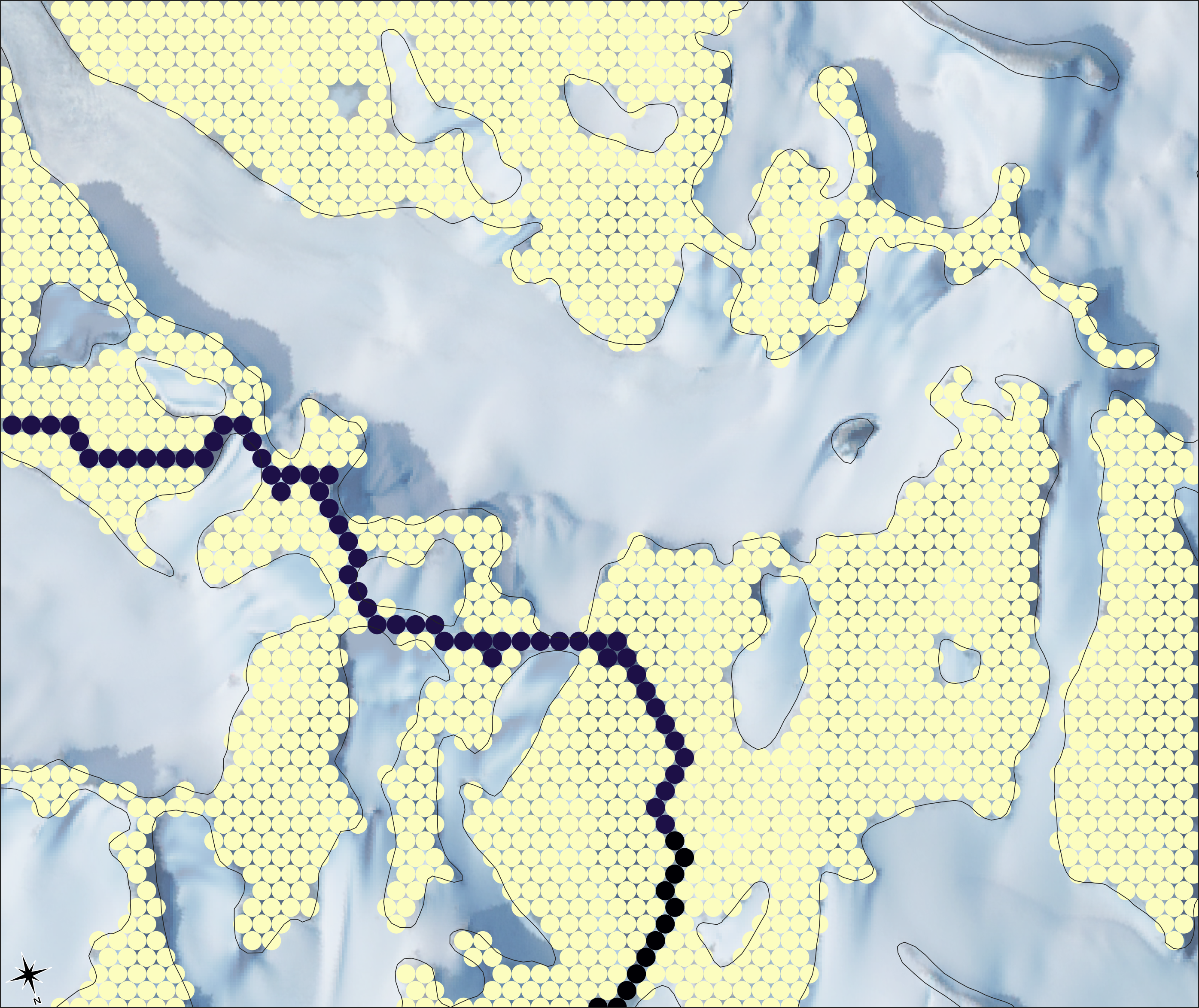
An example output for the largest area of interest is shown below.

r1 <- st_read(str_glue("{data_folder}/dry-valleys/output/dry-valleys-01-32m-betweenness-100-2.gpkg"))
r2 <- st_read(str_glue("{data_folder}/dry-valleys/output/dry-valleys-01-32m-betweenness-200-2.gpkg"))
ext <- st_read(str_glue("{data_folder}/broken-connection-extent.gpkg"))

ggplot() +
  geom_sf(data = r1, aes(colour = cost_vb), size = 0.025) +
  scale_colour_viridis_c(option = "A", direction = -1) +
  theme_void()

This result was obtained at nominal resolution of the hiking network 100m. A coarser grained network, nominal resolution 200m yields a similar result

ggplot() +
  geom_sf(data = r2, aes(colour = cost_vb), size = 0.05) +
  scale_colour_viridis_c(option = "A", direction = -1) +
  geom_sf(data = ext, alpha = 0.35) +
  theme_void()

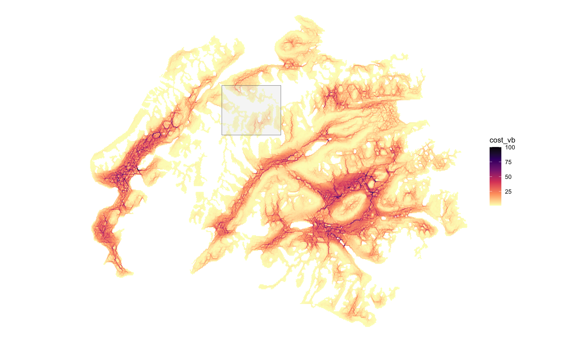
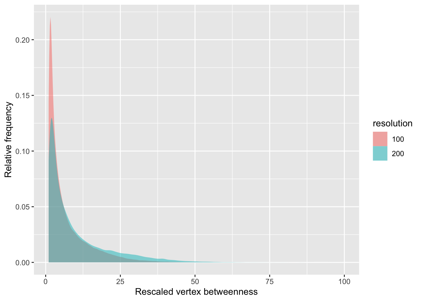
Both results were obtained with a betweenness centrality calculation cutoff of 2 hours estimated hiking time. The resulting beweenness measures have been rescaled in both cases to a range between 1 and 100 to enable direct comparison. The distribution of the results in each case is similar, although the finer resolution network yields more strongly concentrated outcomes.

Code

df <- bind_rows(r1, r2) |>
  mutate(resolution = as.factor(resolution))

ggplot() +
  geom_density(data = df, aes(x = cost_vb, fill = resolution, group = resolution), linewidth = 0, alpha = 0.5) +
  xlab("Rescaled vertex betweenness") +
  ylab("Relative frequency")

However, it is worth noting that there are differences on closer inspection. The area highlighted in the second map above is shown below screenshotted from QGIS.

There are actually two spots here where the image on the right (200m resolution network) is disconnected relative to the 100m resolution case. Note how the 100m resolution network finds two paths through this region, where the 200m resolution network does not. The second ‘missing’ node is towards the top right of the image.

It would not be difficult to fix this by buffering the geology as required, but it may be that such narrow connections are not ‘really’ connections at all…

Footnotes

Mouginot, J., Scheuchl, B. & Rignot, E. MEaSUREs Antarctic Boundaries for IPY 2007-2009 from Satellite Radar, Version 2. 2017, Distributed by NASA National Snow and Ice Data Center Distributed Active Archive Center. https://doi.org/10.5067/AXE4121732AD. Date Accessed 09-03-2024.↩︎
Howat, Ian, et al., 2022, “The Reference Elevation Model of Antarctica – Mosaics, Version 2”, https://doi.org/10.7910/DVN/EBW8UC, Harvard Dataverse, V1, Accessed: 28-29 August 2024.↩︎
Cox SC, B Smith Lyttle, S Elkind, CS Smith Siddoway, P Morin, G Capponi, T Abu-Alam, M Ballinger, L Bamber, B Kitchener, L Lelli, JF Mawson, A Millikin, N Dal Seno, L Whitburn, T White, A Burton-Johnson, L Crispini, D Elliot, S Elvevold, JW Goodge, JA Halpin, J Jacobs, E Mikhalsky, AP Martin, F Morgan, J Smellie, P Scadden, and GS Wilson. 2023. The GeoMAP (v.2022-08) continent-wide detailed geological dataset of Antarctica.PANGAEA. doi: 10.1594/PANGAEA.951482.↩︎