04 Bad Map

Let’s get this over with.

Libraries

Code

library(sf)
library(tmap)
library(dplyr)
library(ggplot2)

Data wrangling

Code

sh1 <- st_read("data/sh1.gpkg") %>%
  st_transform(4326) %>%
  select(geom) %>%
  mutate(Mode = "Road")
interislander <- st_read("data/interislander.gpkg") %>%
  st_transform(4326) %>%
  select(geom) %>%
  mutate(Mode = "Boat")
combined <- sh1 %>%
  bind_rows(interislander) %>%
  mutate(Mode = as.factor(Mode))

The maps

New Zealand’s mighty State Highway 1 (one of the world’s better road trips). I wouldn’t start from here.

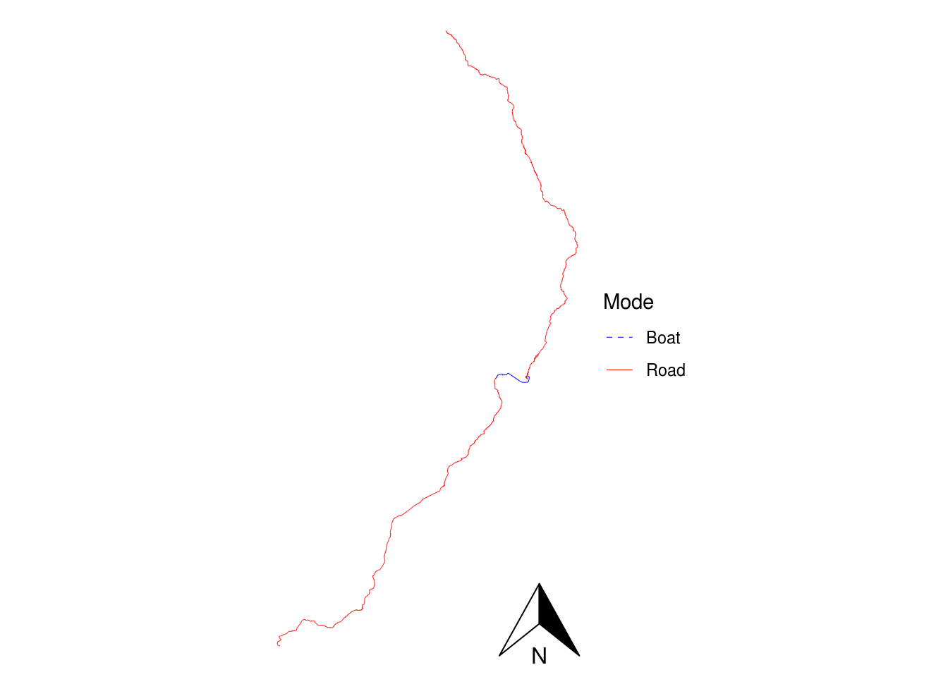
`tmap`

In this example, I wanted to get a better handle on how the legend options work in tmap v4. The tm_legend_combine function is a nice feature, which combines the two symbolisations of colour and line style.

tm_shape(combined) +
  tm_lines(
    col = "Mode",
    col.scale = tm_scale_categorical(
      values = c("blue", "red")),
    lty = "Mode",
    lty.scale = tm_scale_categorical(
      values = c("dashed", "solid")),
    lty.legend = tm_legend_combine("col"),
    lwd = 0.5) +
  tm_layout(
    frame = FALSE,
    legend.frame = FALSE,
    legend.outside = TRUE) +
  tm_compass()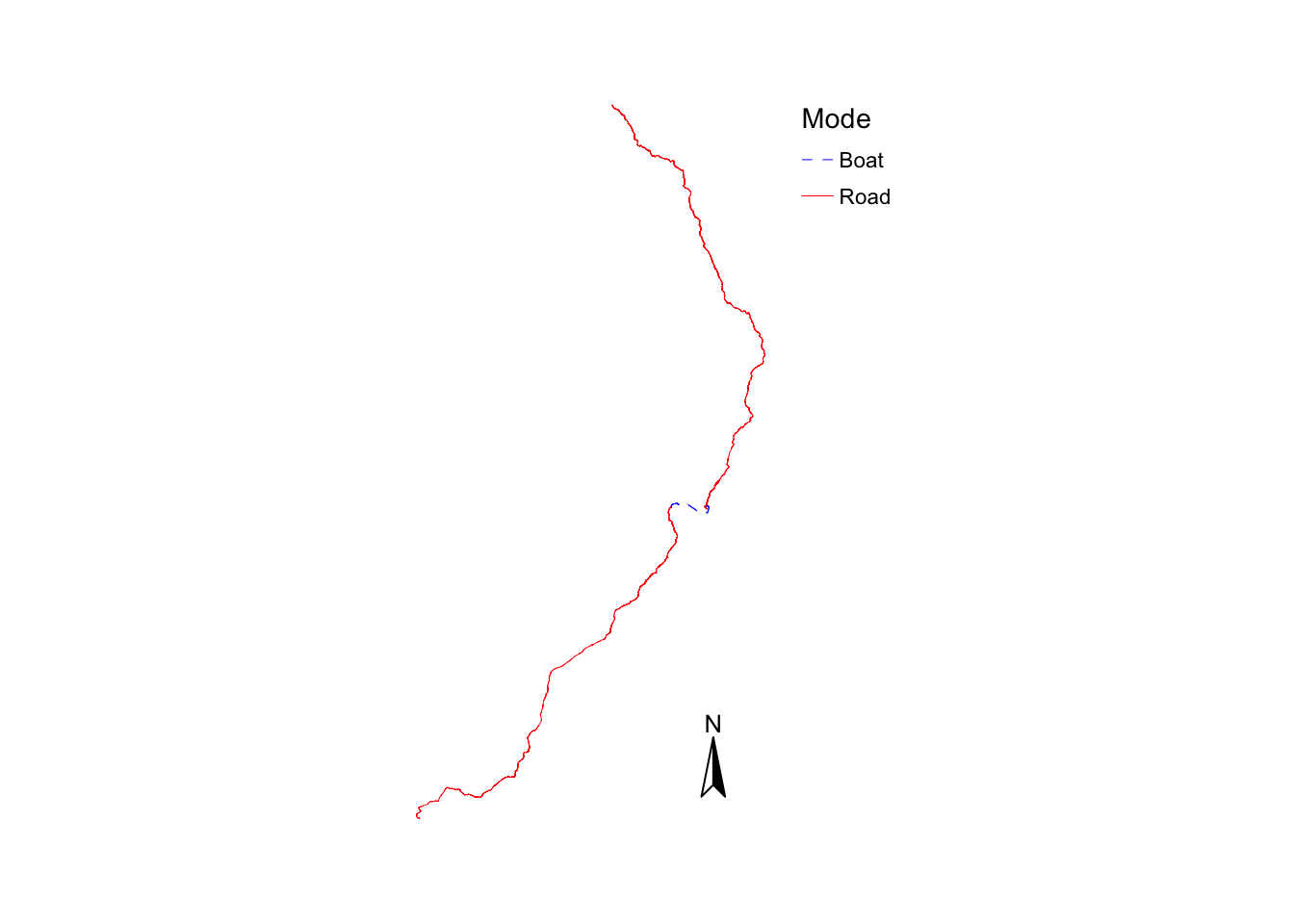

`ggplot2`

Here we need an additional package for the entirely useless north arrow.

ggspatial can do it and seems preferable to the not-very-configurable ggsn. The configurability of ggspatial is a bit over the top for a simple map like this one. On the other hand its default north arrow is very on brand for the theme “Bad Map”!

library(ggspatial)

ggplot(combined) +
  geom_sf(aes(colour = Mode, linetype = Mode), 
              linewidth = 0.5 * 25.4 / 72.27) +
  scale_colour_manual(values = c("blue", "red")) +
  scale_linetype_manual(values = c("dashed", "solid")) +
  annotation_north_arrow(location = "br") + 
  theme_void()