26 Minimal

Less is more.

Probably not really in keeping with the theme for this one, but I once claimed (in Geographical Information Analysis) that a recognisable map of Australia could be formed from only 9 points (sorry Tasmania…). For this theme, I thought I’d take a look at what a minimal New Zealand might look like. Funny thing is, I think you need more points for a recognisable New Zealand.

The source is this Statistics NZ SA2 geographic boundaries dataset selecting only the mainland and island areas, and dissolving them into a single multipolygon. This has around 880,000 vertices. There are a lot of small islands in this dataset (over 1700) and these are rapidly sacrificed by the generalisation process. It is worth noting that R hangs when trying to plot this layer ungeneralised, at least on my laptop (even with 64GB of RAM).

Anyway, to tackle this, I used the rmapshaper package which can do topological simplification of polygons. You specify a keep parameter for the fraction of vertices to retain in the simplified geometries. For reasons of binary division, I started from 5.12% (the ms_simplify function defaults to 5%) and progressed in steps of 50%, all the way down to retaining 0.0025%. At 1 vertex in 40,000 or so of the original geometry we get quite a nice 25 vertex ‘minimal’ New Zealand. After that things start to go a bit pear-shaped (almost literally) as I show at the end of this page.

Stewart Island survives until 0.01% a step more than Lake Taupō, while the Chathams drop out a step before that.

Libraries

library(sf)
library(rmapshaper)
library(tmap)
library(ggplot2)
library(dplyr)

Data wrangling

The two main pain points here are, first, that it is much faster to iteratively apply keep = 0.5 to each step, than to start with the full map and keep 5.12%, then 2.56%, then 1.28% and so on; and second, that getting the factor order right is fiddly. I wanted the facet plots to proceed from less generalised (higher % values) to more, and that requires care in setting up the factor.

nz <- st_read("data/nz-large.gpkg")

start_fraction <- 0.0512
num_steps <- 12

geoms <- c(nz$geom %>% ms_simplify(start_fraction))
for (i in 2:num_steps) {
  geoms <- c(geoms,
             geoms[i-1] %>% ms_simplify(keep = 0.5))
}
percents <- paste(
  start_fraction * 100 * (0.5 ^ (1:num_steps - 1)), "%", sep = "")

nzs <- 
  data.frame(
    Percent = ordered(percents, levels = percents), 
    geom = geoms %>% st_sfc()) %>%
  st_as_sf()

The maps

tmap

This case lets us see how tm_facets works. Pretty simple really. free.coords = FALSE is necessary to make sure the panels are all scaled the same.

tm_shape(nzs) + 
  tm_polygons(col = "black") +
  tm_layout(main.title = "Generalisation % of vertices retained") +
  tm_facets(by = "Percent", ncol = 4, free.coords = FALSE)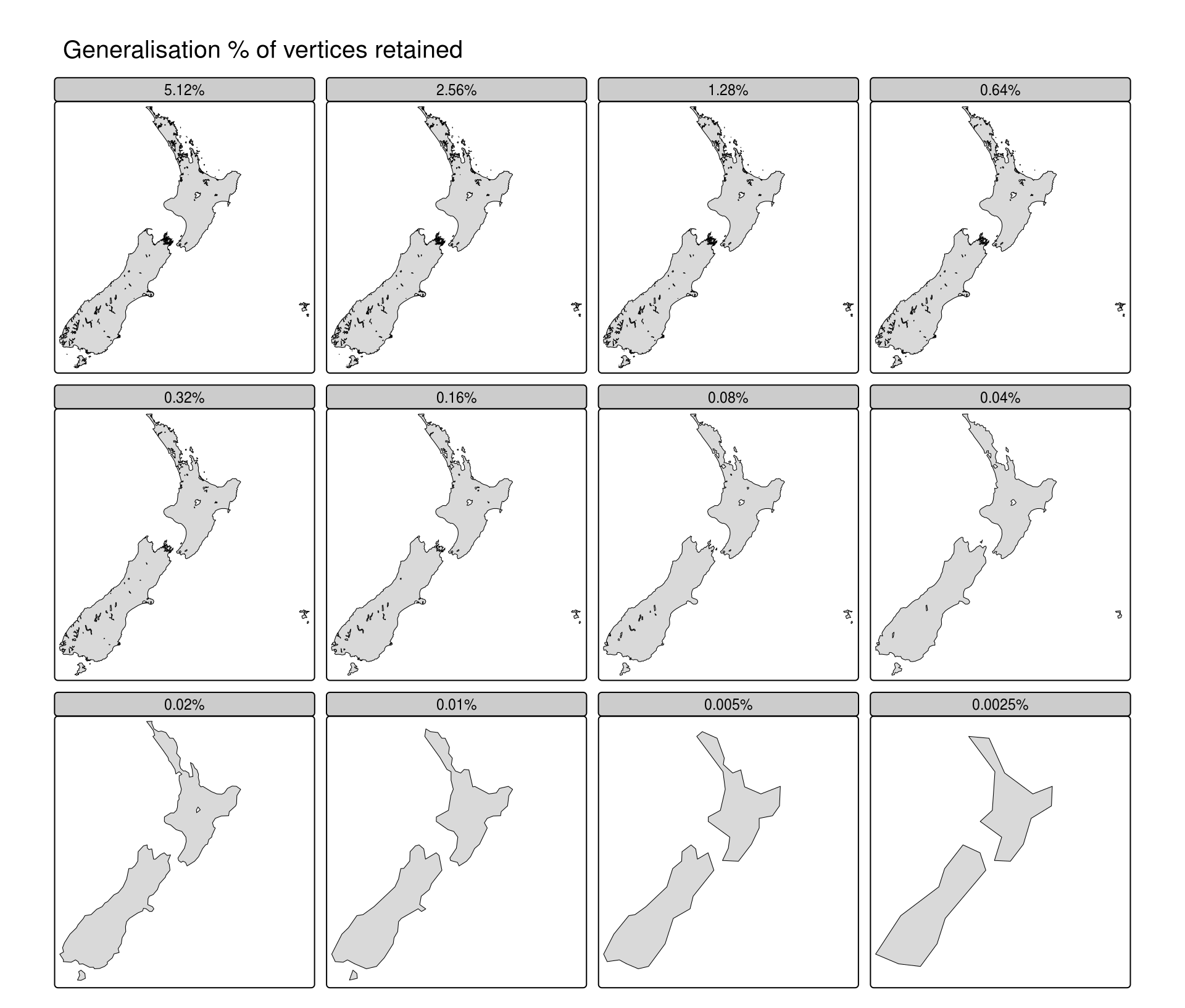

ggplot2

facet_wrap handles this very nicely.

ggplot(nzs) +
  geom_sf(linewidth = 25.4 / 72.27) +
  facet_wrap( ~ Percent, ncol = 4) + 
  labs(title = "Generalisation % of vertices retained") +
  theme_void() +
  theme(panel.border = element_rect(fill = NA))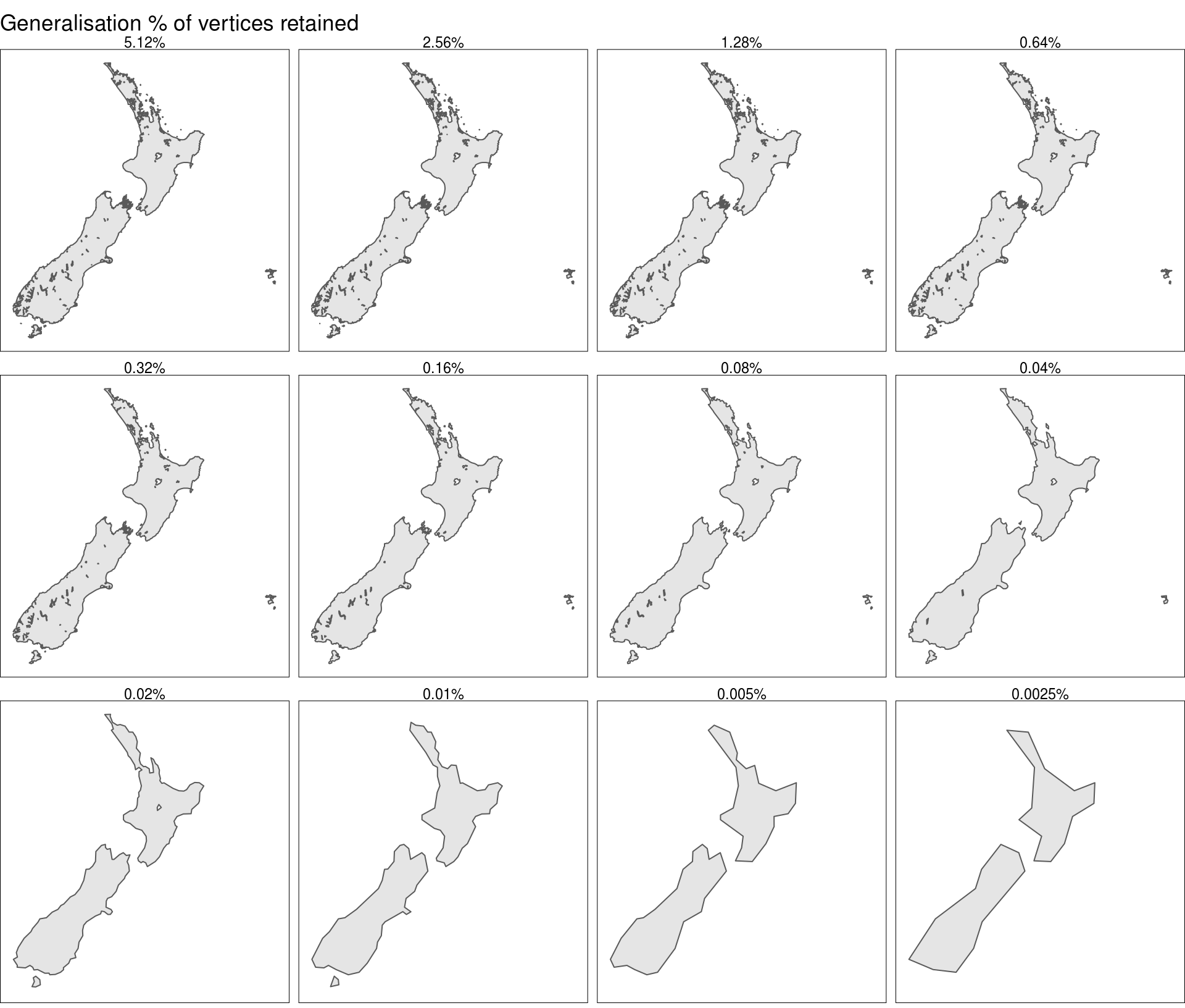

So… here’s a pretty recognisable minimal map of New Zealand, with 25 points:

plot(geoms[12])

One more step and it gets pretty bad:

plot(geoms[12] %>% 
       ms_simplify(keep = 0.5))

One more gets us an unexpectedly recognisable 10 vertices:

plot(geoms[12] %>% 
       ms_simplify(keep = 0.5) %>% 
       ms_simplify(keep = 0.5))

After that it really doesn’t work:

plot(geoms[12] %>% 
       ms_simplify(keep = 0.5) %>% 
       ms_simplify(keep = 0.5) %>% 
       ms_simplify(keep = 0.5))