06 Asia

Libraries

Code

library(sf)
library(tmap)
library(dplyr)
library(stringr)
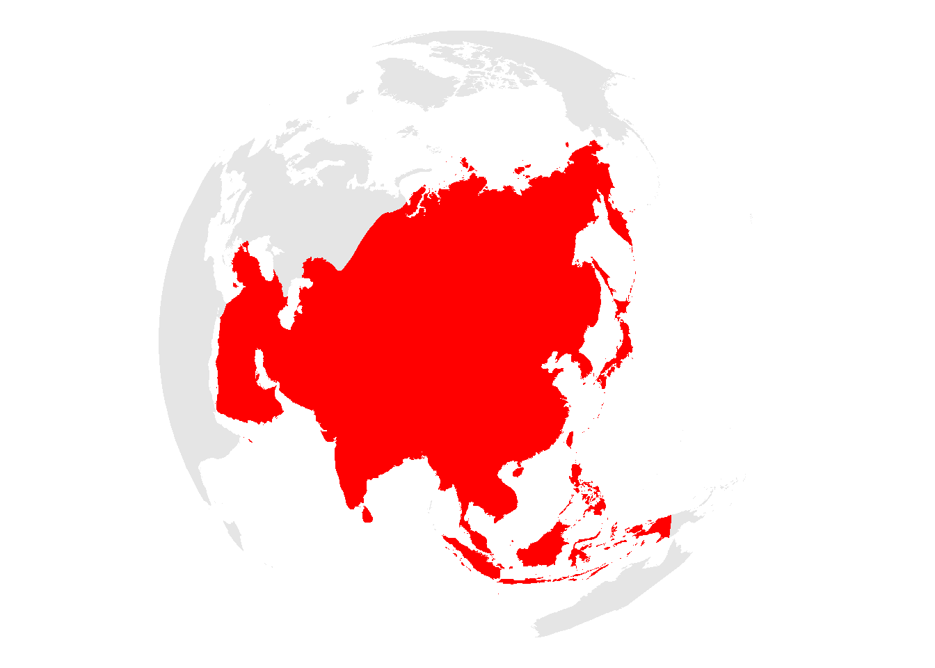
library(ggplot2)

Largest of the continents.

The ‘continent’ series

Along with this one, Days 8, 10, 12, 14, 16, and 25 are each one of the seven continents. I’ve mapped them all the same way, so all the commentary is on this page.

There’s not much to say here. The biggest challenge in this case was finding a latitude-longitude coordinate pair for the centre of the orthographic projection that didn’t result in lost polygons or some other distortion of the geometry. The only fix was to hunt around a bit in the vicinity of the ‘centre’ of each continent. That’s also why there is a post-projection st_make_valid() followed by a filter(!st_is_empty(.)) to handle some simpler cleanups. In the absence of these tmap in particular is unhappy to map the data.

For what it’s worth, the built in data(World) that accompanies tmap was more prone to these issues than the Natural Earth dataset I’ve used.

Both tmap and ggplot2 handle this style of map admirably, with little fuss. I’ve suppressed the graticule because these often showed problems in the orthographic projection (more on this in a later map.)

Data wrangling

Code

focus <- "Asia"
lon0 <- 100
lat0 <- 45
proj <- str_glue("+proj=ortho lon_0={lon0} lat_0={lat0}")

world <- st_read("data/ne_110m_admin_0_map_units.gpkg") %>%
  st_make_valid() %>%
  select(CONTINENT)

world_o <- world %>%
  st_transform(proj) %>%
  st_make_valid() %>%
  filter(!st_is_empty(.)) %>%
  group_by(CONTINENT) %>%
  summarise() 

continent <- world %>%
  filter(CONTINENT == focus)

The maps

`tmap`

tm_shape(world_o) +
  tm_fill() + 
  tm_shape(continent) +
  tm_fill(fill = "red") +
  tm_layout(frame = FALSE)

`ggplot2`

ggplot(world_o) +
  geom_sf(linewidth = 0) +
  geom_sf(
    data = continent, 
    fill = "red", 
    linewidth = 0) +
  theme_void()