Code
library(sf)
library(tmap)
library(dplyr)
library(ggplot2)Classic thematic map: a choropleth.
This one is where tmap comes into its own, although v4 in increasing the available options requires more code to make the same map compared to v3.
ggplot2 by contrast is allergic to making classic classified choropleth maps, so much so that it’s quite hard to imagine using it in any kind of introductory teaching setting. Having to explicitly make the classification using the not-very-friendly classInt package is a layer of complexity which tmap shields the user from.
I think a lot of users would very much appreciate an addition to the ggplot2-verse that could handle classifying data according to the various styles offered by classInt (in effect wrapping classInt as does tmap).
library(sf)
library(tmap)
library(dplyr)
library(ggplot2)ak <- st_read("data/ak-demographics-2018.gpkg") %>%
slice(-1) # remove Gulf Islands
nz <- st_read("data/nz.gpkg")tmapThe idea behind the tmap v4 semantics makes complete sense, but it is quite verbose. It is nice to have the additional control that the separate specification of the .scale and .legend parameters provide, but the downside is a lot of additional typing. On the other, hand, if you like typing, take a look at what’s involved in making a similar map using ggplot2.
Some of the additional difficulty here is choosing to use a ‘non-standard’ legend, but this still seems like quite a lot of code.
tm_shape(nz, bbox = ak) +
  tm_fill(fill = "lightgray") +
  tm_shape(ak) +
  tm_polygons(
    fill = "maori",
    fill.scale = tm_scale_intervals(
      n = 9, values = "YlGnBu", style = "quantile"),
    fill.legend = tm_legend(
      orientation = "landscape", title = "% Māori"),
    col = "grey",
    lwd = 0.35
  ) +
  tm_layout(
    frame = FALSE, legend.outside = TRUE,
    legend.outside.position = "bottom",
    legend.frame = FALSE)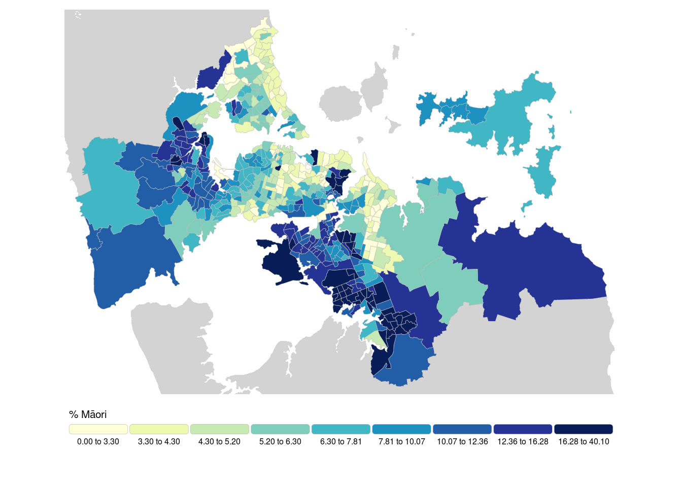
Version 3.x tmap would accomplish the same map (focusing only on the two layers and their styling) with
tm_shape(nz) +
  tm_fill(fill = "lightgray") +
  tm_shape(ak) +
  tm_polygons(col = "maori", n = 9, palette = "YlGnBu",
              style = "quantile", border.col = "grey", lwd = 0.35)
I should note that at least for now this v3 code will be internally transformed to v4 code, and hence still directly useable.
The ‘embedded functions’ approach such as tm_scale_intervals seems like extra work. The change from palette to values is consistent with the visual variables concept, but I think you have to admit that it may be less obvious to a beginner.
ggplot2Here, we have to do all the classification work and use the scale_fill_fermenter() function to get the same effect. We use classInt::classIntervals() to make breaks. Even then we have to make up the legend labels manually if we want to show ranges, not just the break values. Much as I appreciate the uh… quirkiness of R’s paste() function, I don’t relish explaining this to an introductory class!
An additional challenge caused by placing the legend below the map area is that we have to extend the plot area to accommodate it, using coord_sf(...ylim=...), but that’s a distraction, it is the generation of breaks, and legend labels that is the real annoyance (at least to me).
library(classInt)

class_breaks <- classIntervals(ak$maori, 9, "quantile", digits = 1)
brks <- round(class_breaks$brks, 1)
intervals <- paste(brks[-10], rep("to", 9), brks[-1])

# A lot of fiddle here to allow for both clipping NZ appropriately
# and expanding the map area to accommodate a legend below it
bb <- st_bbox(ak) %>%
  st_as_sfc(crs = 2193) %>%
  st_sf()
# we need to clip with an oversize bounding box - unfortunately using
# a buffer leads to rounded or mitred corners
ctr <- st_centroid(bb)
clip <- (bb - ctr) * matrix(c(1.05, 0, 0, 1.05), 2, 2) + ctr
clip <- clip$geometry %>%
  st_sfc(crs = 2193) %>%
  st_sf()
bb <- st_bbox(bb)

ggplot(nz %>% st_intersection(clip)) +
  geom_sf(fill = "lightgray", linewidth = 0) +
  geom_sf(data = ak, aes(fill = maori), colour = "grey",
          linewidth = 0.35 * 25.4 / 72.27) +
  scale_fill_fermenter(
    palette = "YlGnBu",
    direction = 1,
    breaks = brks[-10],
    labels = intervals,
    name = "% Māori",
    guide = guide_legend(nrow = 1,
      keywidth = unit(15, units = "mm"),
      keyheight = unit(3, units = "mm"),
      label.position = "bottom", title.position = "top")) +
  coord_sf(ylim = c(bb[2] - 1e4, bb[4]), expand = FALSE) +
  theme_void() +
  theme(legend.position = c(0.5, 0.1))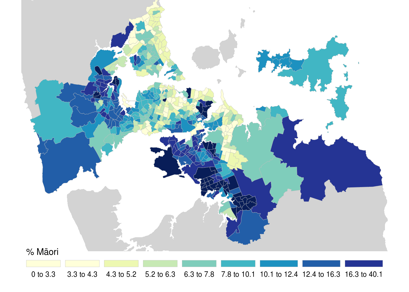
The underlying issue here is that ggplot2 really doesn’t want to make classed choropleths. The data are ‘continuous’ valued and ggplot2’s strong preference is to associate a continuous variable with a continuous visual variable. You can see this if you let it do its own thing:
ggplot(nz %>% st_intersection(clip)) +
  geom_sf(fill = "lightgray", linewidth = 0) +
  geom_sf(data = ak, aes(fill = maori), colour = "grey",
          linewidth = 0.35 * 25.4 / 72.27) +
  scale_fill_distiller(palette = "YlGnBu", direction = 1) +
  theme_void()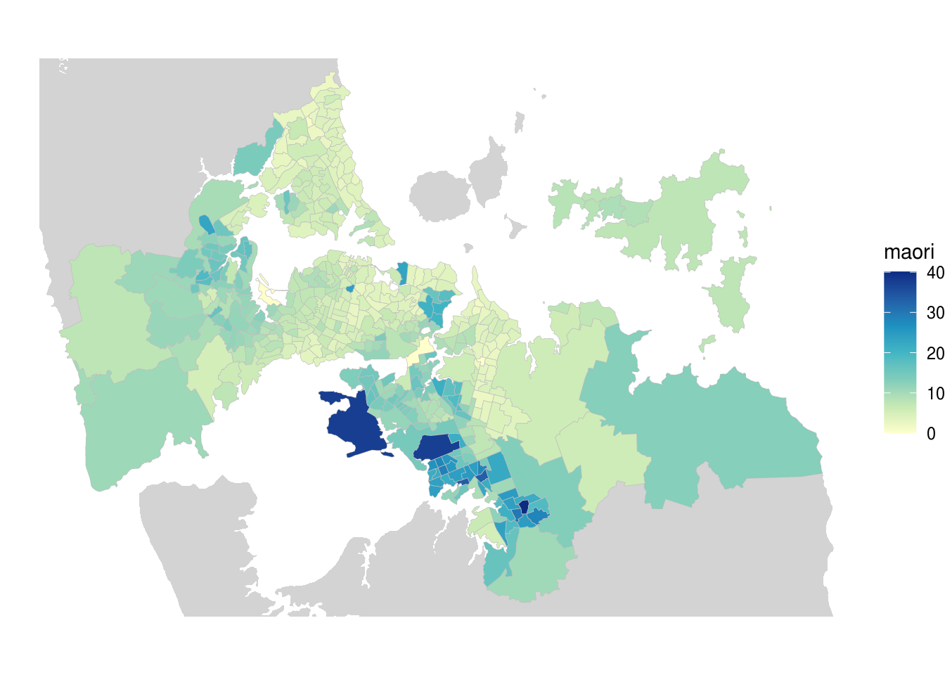
Data values are mapped directly to positions on the colour ramp. Doing different things to this requires the kind of additional work we see above.
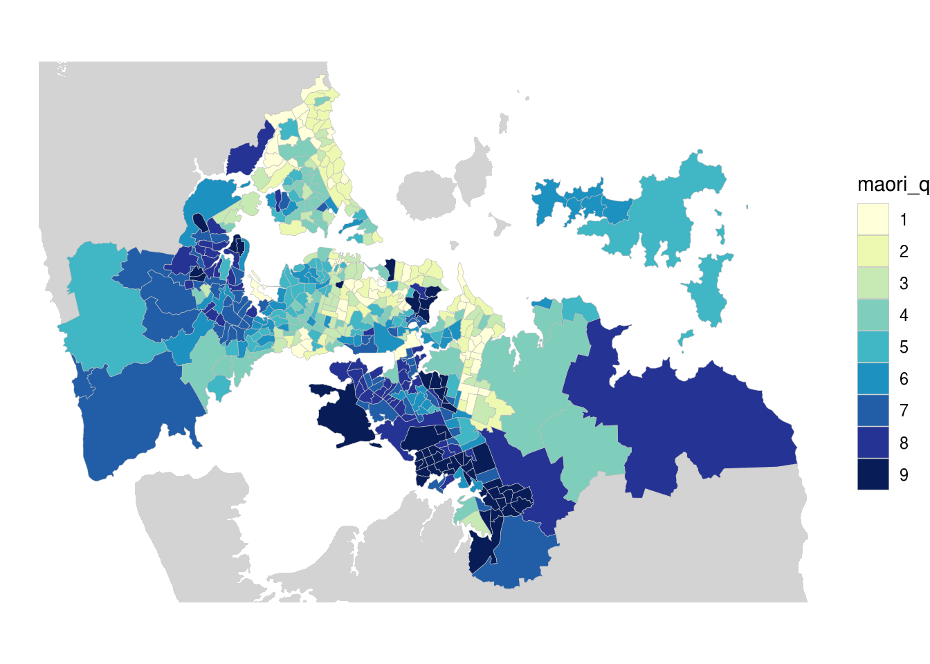
ggplot2An alternative approach that gets close to the end-goal, but will only work for a quantile mapping scheme is to use the dplyr::ntile function. However, this still leaves plenty of work to do getting break points for an informative legend, so in this situation it’s not that much help.
It also doesn’t help at all for other classification schemes. It also prioritises making buckets equal-sized over putting cases in the right bucket, so that areas with the same value might end up in different buckets if they happen to sit on a class interval boundary!
So… not really a fix at all.
I haven’t bothered with cleaning up the legend here, which also shows how this is only a very partial workaround. Worth knowing about, but perhaps not as useful at it first appears.
ak <- ak %>%
  mutate(maori_q = as.factor(ntile(maori, 9)))

ggplot(nz %>% st_intersection(clip)) +
  geom_sf(fill = "lightgray", linewidth = 0) +
  geom_sf(data = ak, aes(fill = maori_q), colour = "grey",
          linewidth = 0.35 * 25.4 / 72.27) +
  scale_fill_brewer(palette = "YlGnBu") +
  theme_void()