17 Flow

Flow of transport, people.

Well… no, flow of water.

Data for the Manawatū catchment in Te Ika-a-Māui is from the NZ Ministry for the Environment, and available at koordinates.com.

Elevation data is a 25m resolution DEM from Manaaki Whenua Landcare Research, which I had kicking around on my laptop. Clearly getting a bit long in the tooth as it was for some reason in the old NZ Map Grid (EPSG 27200) projection and had to be reprojected to NZ Transverse Mercator (EPSG 2193).

Libraries

Code

library(terra)
library(tidyterra)
library(sf)
library(ggplot2)
library(tmap)

Data wrangling

I wanted to use a hillshaded DEM in this one. It was feasible in tmap to layer a hypsometric coloured DEM and a hillshade derived from it in terra easily enough. In ggplot2 it proved a problem because having more than one map layer attempt to use the fill aesthetic is verboten. I am sure there is a way around this, but while 30 days is a long time, sometimes life is too short for hunting around on stackoverflow, so it was easier to jump out to the excellent (and free) PyramidShader and do the work there to make a hillshaded and coloured DEM image. That still required a bit of fiddle to make it work in the two tools I’m using, but nothing too difficult.

The successor to PyramidShader, Eduard looks excellent, but not worth me buying for this project alone!

Code

nz <- st_read("data/nz.gpkg")
flows <- st_read("data/manawatu-flows.gpkg") 
# %>%
#   dplyr::arrange(desc(ORDER))
catch <- st_read("data/manawatu-catch.gpkg")

mask <- catch %>%
  st_buffer(2.5e3, nQuadSegs = 0) %>%
  st_bbox() %>%
  st_as_sfc(crs = 2193) %>%
  st_sf() %>%
  st_difference(catch) %>%
  st_intersection(nz)

hillshaded_dem <- rast("data/manawatu-dem-rect-image.tif") %>%
  tidyterra::select(1:3) %>%
  crop(nz %>% as("SpatVector"), mask = TRUE)
terra::set.crs(hillshaded_dem, "epsg:2193")
names(hillshaded_dem) <- c("r", "g", "b")

bbox <- catch %>%
  st_buffer(2.5e3) %>%
  st_bbox()

The maps

Per this issue tm_scalebar at time of writing tmap fails with tm_pos_out for placing the scale bar outside the map area.

tmap seems to run quite slowly with raster layers.

In general however, tmap is the winner in this comparison because it can cope with multiple layers using the same aesthetics. For most people making maps, it’s entirely natural to assume you can style them independently of one another and layer them on top of each other. Just because one layer uses the fill colour aesthetic doesn’t mean that no other layer can also use it, which is what happens in ggplot2’s world.

`tmap`

tm_shape(hillshaded_dem, bbox = bbox) +
  tm_rgb(tm_mv("r", "g", "b")) +
  tm_shape(mask) +
  tm_fill(fill = "white", fill_alpha = 0.35) +
  tm_shape(flows) + 
  tm_lines(
    lwd = "ORDER", 
    lwd.scale = tm_scale_discrete(values.scale = 2),
    lwd.legend = tm_legend(title = "Stream order"),
    col = "MeanFlowCumecs", 
    col.scale = tm_scale_continuous_log(
      values = RColorBrewer::brewer.pal(9, "Blues")[3:9]),
    col.legend = tm_legend(title = "Flow cubic m/sec")) +
  tm_title("Manawatū catchment") +
  tm_scalebar() +
  # position = tm_pos_auto_out(
  # cell.h = "center", cell.v = "bottom",
  # pos.h = "right", pos.v = "top")) +
  tm_layout(legend.frame = FALSE, bg.color = "lightblue2")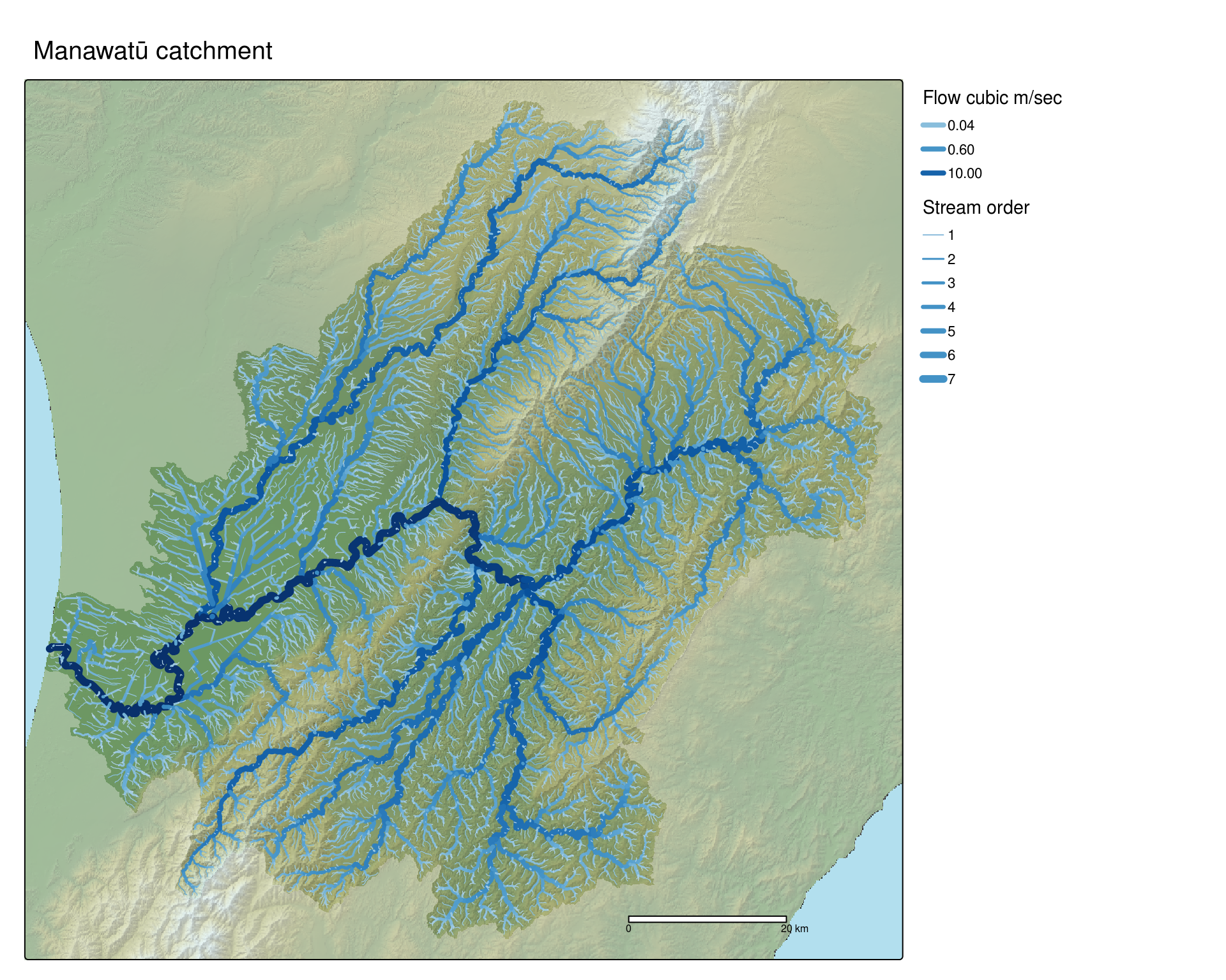

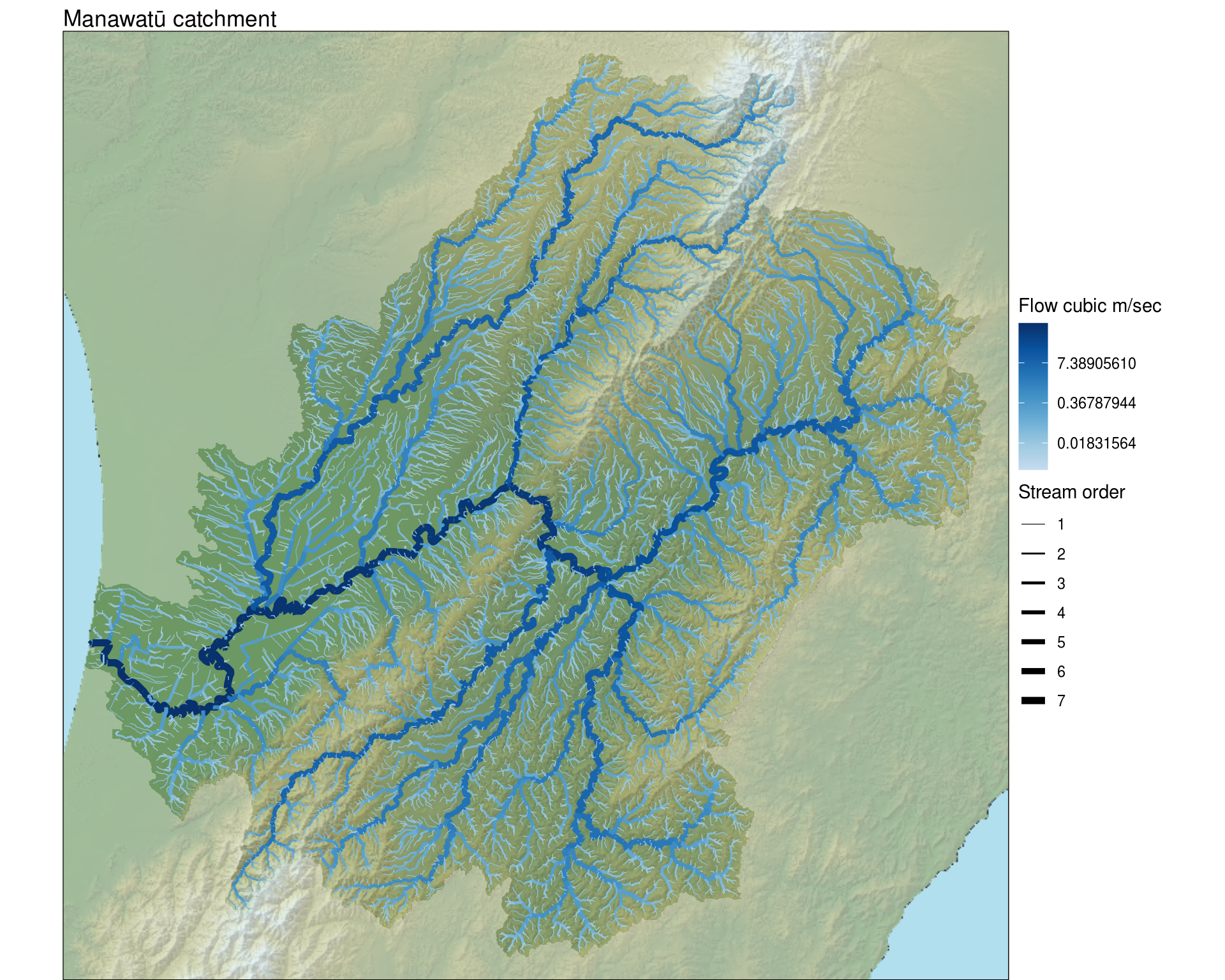
`ggplot2`

ggplot2 is unwilling to handle two rasters layered on top of one another as both are trying to use the fill aesthetic, but that was resolved by generating the hillshade relief in an external tool. Even then, the tidyterra package proved a much better bet for deploying a raster layer in ggplot2 than anything native.

I could add a scale bar and whatnot using ggspatial as I have in other maps, but honestly… I’ve had enough of this foray into more ‘topographic’ as opposed to ‘thematic’ mapping for now, so I’ll leave that as an exercise for the reader.

library(tidyterra)

ggplot() +
  geom_spatraster_rgb(data = hillshaded_dem) +
  geom_sf(data = flows, 
          aes(colour = MeanFlowCumecs, linewidth = ORDER)) +
  geom_sf(data = mask, fill = "white", alpha = 0.35, linewidth = 0) +
  scale_linewidth(range = c(0.2, 2), name = "Stream order") +
  scale_colour_gradientn(
    colours = RColorBrewer::brewer.pal(9, "Blues")[3:9],
    name = "Flow cubic m/sec", trans = "log") +
  coord_sf(xlim = bbox[c(1, 3)], ylim = bbox[c(2, 4)], 
           expand = FALSE) +
  ggtitle("Manawatū catchment") +
  theme_void() +
  theme(panel.background = element_rect(fill = "lightblue2"),
        panel.border = element_rect(fill = NA, colour = "black"))