24 Black & white

Only two colors allowed.

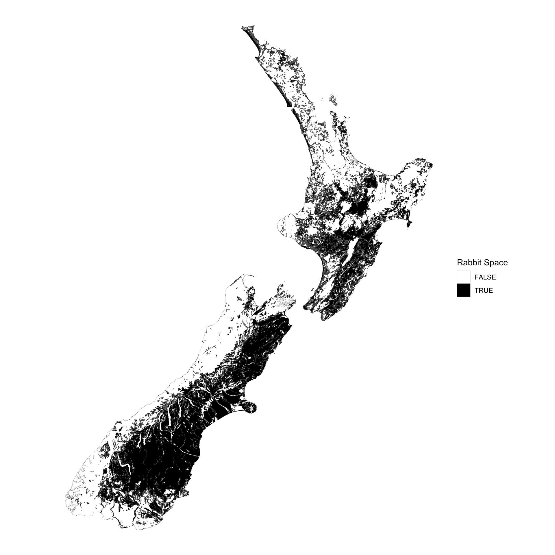
I already did this with 11 Retro and kind of again with 20 Outdoors so once more back to searching for suitable data in Aotearoa New Zealand. In deference to the greatest ever black and white maps—Horvath’s machine space—see

Horvath RJ. Machine space. Geographical Review 64(2) 167-188.

already referenced in map 20, I tried to track down an impervious cover layer for a New Zealand city, any New Zealand city, but without success. You’d maybe think given all the trouble New Zealand has been having with flooding lately that this would be more of a thing… apparently not, although I note that Auckland City have been working with Lynker Analytics on this topic.

Anyway, quite by chance, while on the hunt for impervious cover, New Zealand rabbit proneness came to my attention, and not being one to resist a uh… rabbit hole I fell for it, and here we all are: Rabbit Space.

Libraries

Code

library(sf)
library(tmap)
library(ggplot2)
library(dplyr)

Data wrangling

Code

binary <- data.frame(
  RCODE2 = c("e", "H", "i", "l", "L", "M", "O", "q", "r", "t", "X"),
  rabbit_prone = c(FALSE, TRUE, FALSE, FALSE, TRUE, TRUE, 
                   FALSE, FALSE, FALSE, FALSE, TRUE)
)

dang_rabbits <- st_read("data/rabbits.gpkg") %>% 
  left_join(binary) %>%
  group_by(rabbit_prone) %>%
  summarise()

The maps

`tmap`

tm_shape(dang_rabbits) +
  tm_polygons(
    fill = "rabbit_prone", 
    fill.scale = tm_scale_categorical(
      levels = c(FALSE, TRUE),
      values = c("white", "black")),
    fill.legend = tm_legend(title = "Rabbit Space"),
    lwd = 0.1) +
  tm_layout(frame = FALSE, legend.frame = FALSE)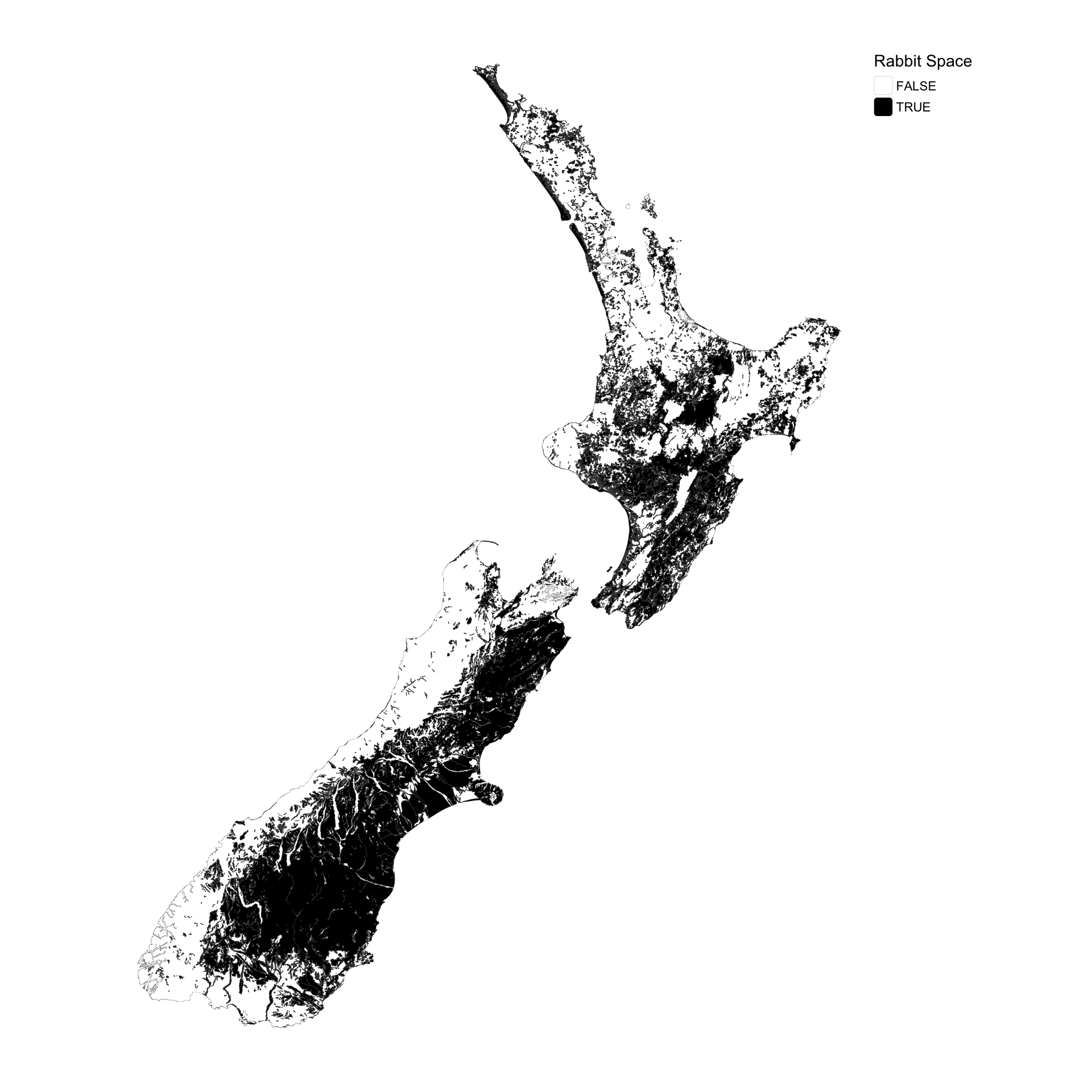

`ggplot2`

ggplot(dang_rabbits) +
  geom_sf(aes(fill = rabbit_prone), linewidth = 0.1 * 25.4 / 72.27) +
  scale_fill_manual(values = c("white", "black"), 
                    name = "Rabbit Space") +
  theme_void()