20 Outdoors

Map of mountains, trails, or something completely different.

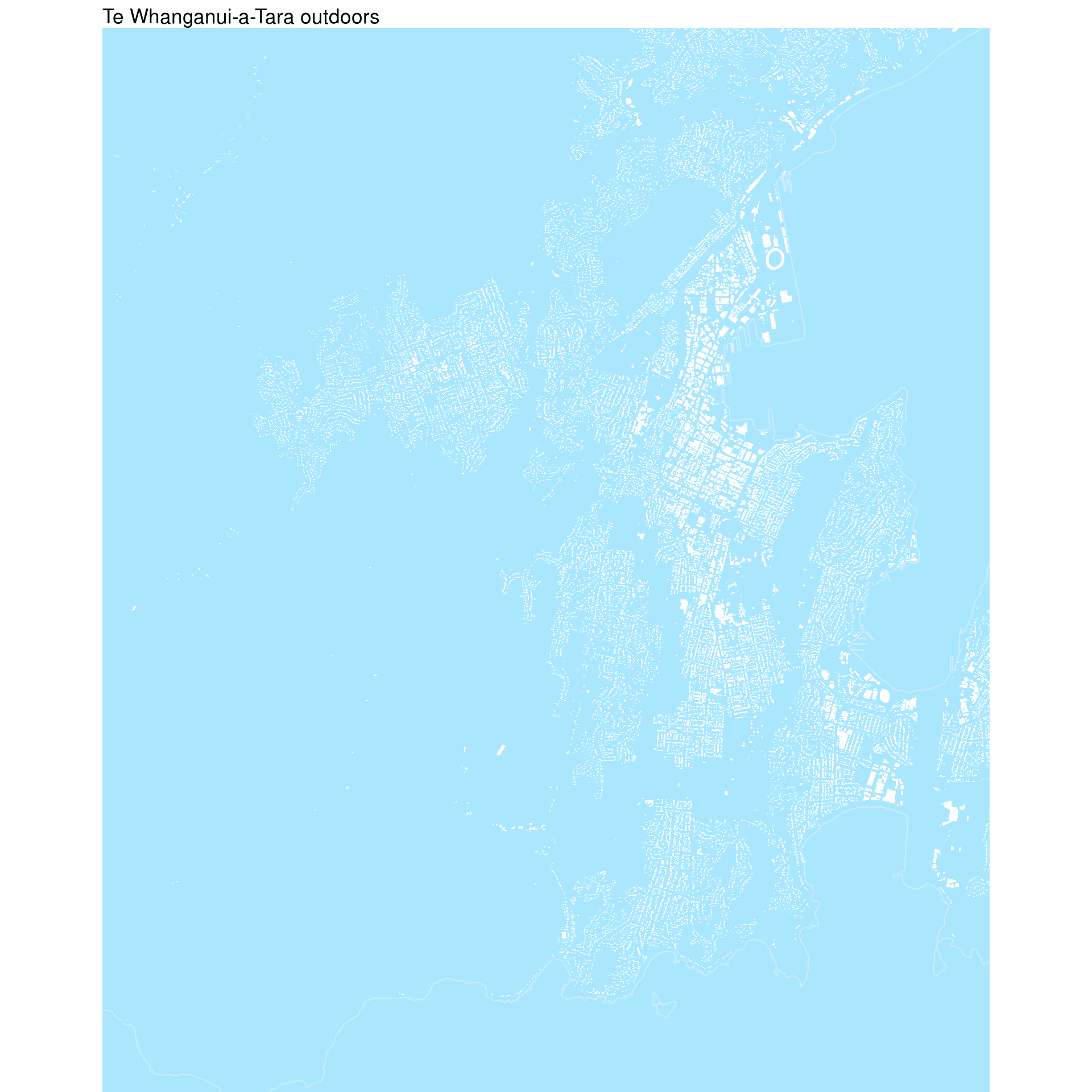
As previously noted much of the outdoors in Wellington is dominated by wind.

That’s why I’ve used a pale blue for all of the space outside the buildings in these maps. If it was a warmer time of year, that blue might be a bit less watery and cold.

The visual inspiration is machine space

Horvath RJ. Machine space. Geographical Review 64(2) 167-188.

but inverted. Of course, a lot of the ‘open’ space here is also machine space (given over to cars), but still, it’s fun to look a the built environment in this way.

The buildings are from Te Toitū Whenua - Land Information New Zealand.

But the buildings aren’t the spatial dataset here: outdoors.gpkg is a rectangle of the extent of the map with holes punched out where the buildings (the ‘indoors’) are. So it’s a ‘outdoors’ polygon. You can’t really tell that from the map, but the white areas are the background colour showing through the holes.

Libraries

Code

library(sf)
library(tmap)
library(ggplot2)

Data wrangling

Code

outdoors <- st_read("data/outdoors.gpkg")
coast <- st_read("data/welly-outdoors-coast.gpkg")

The maps

`tmap`

tm_shape(outdoors) +
  tm_fill(fill = "#aae7ff") +
  tm_shape(coast) +
  tm_lines(col = "#cceeff") +
  tm_title("Te Whanganui-a-Tara outdoors",
    position = tm_pos_out(
      cell.h = "center", cell.v = "top",
      pos.h = "left", pos.v = "top")) +
  tm_layout(frame = FALSE, inner.margins = rep(0, 4))

`ggplot2`

library(ggspatial)

ggplot() +
  geom_sf(data = outdoors, fill = "#aae7ff", linewidth = 0) +
  geom_sf(data = coast, colour = "#cceeff",
          linewidth = 25.4 / 72.27) +
  coord_sf(xlim = st_bbox(outdoors)[c(1, 3)],
           ylim = st_bbox(outdoors)[c(2, 4)],
           expand = FALSE) +
  ggtitle("Te Whanganui-a-Tara outdoors") +
  theme_void()