09 Hexagons

6 sides, 6 angles, and 6 vertices.

Wishing to use a static web basemap increased the degree of difficulty here.

Having said that, tmap’s built in tm_basemap() function seems promising and intuitive.

A bit of hunting around suggests that the ggspatial package’s annotation_map_tile() function is the best for basemaps in ggplot2.

Libraries

Code

library(dplyr)
library(h3forr)
library(tmap)
library(sf)
library(ggplot2)
library(stringr)

Data wrangling

Code

square <- c(1.74e6 + 1e4 * c(0, 0, 1, 1, 0), 
            5.42e6 + 1e4 * c(0, 1, 1, 0, 0)) %>%
  matrix(ncol = 2) %>%
  list() %>%
  st_polygon() %>%
  st_sfc() %>%
  st_sf(crs = 2193) %>%
  st_transform(4326)

get_hexes <- function(poly, resolution, distance) {
  poly %>% 
    st_buffer(distance) %>%
    polyfill(res = resolution) %>% 
    h3_to_geo_boundary() %>% 
    geo_boundary_to_sf()
}

h3_5 <- get_hexes(square, 5, 5000) %>% 
  st_cast("LINESTRING")
h3_6 <- get_hexes(square, 6, 2500) %>% 
  st_cast("LINESTRING")
h3_7 <- get_hexes(square, 7, 1500) %>% 
  st_cast("LINESTRING")
h3_8 <- get_hexes(square, 8, 1000) %>% 
  st_cast("LINESTRING")
h3_9 <- get_hexes(square, 9, 750) %>% 
  st_cast("LINESTRING")
h3_10 <- get_hexes(square, 10, 500) %>% 
  st_cast("LINESTRING")

bb <- h3_10 %>% 
  st_union() %>%
  st_bbox()

credit <- maptiles::get_credit("OpenStreetMap")

tm_lwds <- c(3.5, 2.5, 1.5, 1, 0.7, 0.5)
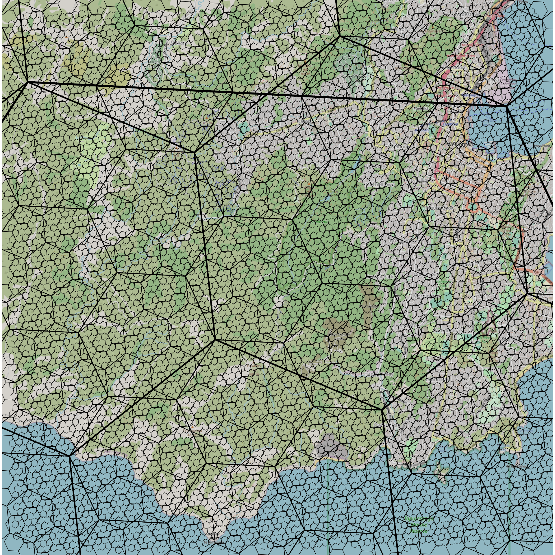
gg_lwds <- tm_lwds * 25.4 / 72.27

The maps

`tmap`

tmap v4 has a built-in web basemap function. The raster downscaling kicks in to make the image a bit unsatisfactory, but I assume that option will be tweakable in due course.

tm_basemap(server = "OpenStreetMap", zoom = 12) +
  tm_shape(h3_5) + 
  tm_lines(lwd = tm_lwds[1]) +
  tm_shape(h3_6) + 
  tm_lines(lwd = tm_lwds[2]) +
  tm_shape(h3_7) + 
  tm_lines(lwd = tm_lwds[3]) +
  tm_shape(h3_8) + 
  tm_lines(lwd = tm_lwds[4]) +
  tm_shape(h3_9) + 
  tm_lines(lwd = tm_lwds[5]) +
  tm_shape(h3_10, is.main = TRUE) + 
  tm_lines(lwd = tm_lwds[6]) +
  tm_credits(
    credit,
    position = tm_pos_out(pos.h = "RIGHT", pos.v = "TOP",
                          cell.h = "center", cell.v = "bottom")) + 
  tm_layout(frame = FALSE)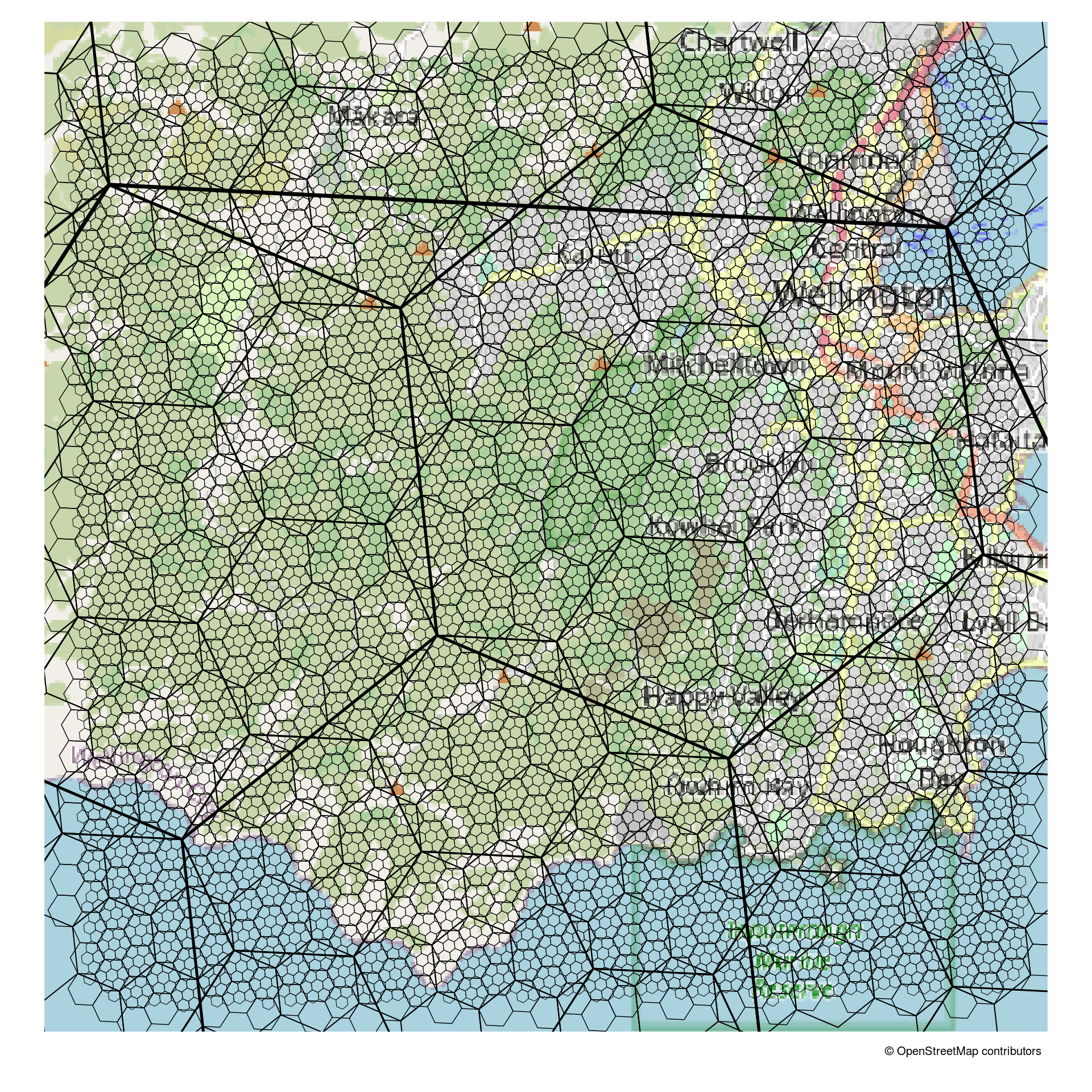

`ggplot2`

ggspatial seems the best option for a static background basemap.

library(ggspatial)

ggplot(square, aes(colour = "#00000000")) +
  annotation_map_tile(zoomin = 1) + 
  geom_sf(data = h3_5, linewidth = gg_lwds[1], colour = "black") +
  geom_sf(data = h3_6, linewidth = gg_lwds[2], colour = "black") +
  geom_sf(data = h3_7, linewidth = gg_lwds[3], colour = "black") +
  geom_sf(data = h3_8, linewidth = gg_lwds[4], colour = "black") +
  geom_sf(data = h3_9, linewidth = gg_lwds[5], colour = "black") +
  geom_sf(data = h3_10, linewidth = gg_lwds[6], colour = "black") +
  ggplot2::coord_sf(
    xlim = bb[c(1, 3)], ylim = bb[c(2, 4)], expand = FALSE) +
  theme_void()