27 Dot

Dot density, a single dot in space or something different.

Definitely something different.

Again, drawing on our weaving space tools, I made a tiled map based on a 7-colouring by hexagons. Symbolising the hexagons with coloured ‘dots’ allows the simultaneous visualisation of seven variables, in this case components of an index of multiple deprivation developed by Dan Exeter and colleagues at University of Auckland. The position of each aspect of the index is shown in the key and all are coloured on a red-white-blue diverging scale, where red indicates higher levels of deprivation on that aspect.

Note that the deprivation levels shown in these maps are for the Auckland Central region, but relative to the distribution across all of New Zealand. That is one reason why many areas are ranked ‘deprived’ with respect to ‘crime’ and ‘housing’ while scoring better on other aspects.

Libraries

Code

library(sf)
library(tmap)
library(dplyr)
library(stringr)

Data wrangling

Code

hexes <- st_read("data/h7-base.gpkg")

layers <- list()
tilesets <- list()
for (id in letters[1:7]) {
  these_hexes <- hexes %>% filter(element_id == id)
  layers[[id]] <- these_hexes 
  tilesets[[id]] <- these_hexes$tile_id
}
tiles <- tilesets[[1]]
for (i in 2:7) {
  tiles <- intersect(tiles, tilesets[[i]])
}
legend_elements <- hexes %>% 
  select(geom, tile_id, element_id) %>%
  filter(tile_id == tiles[1])

base <- hexes %>% 
  select(geom, tile_id) %>%
  group_by(tile_id) %>%
  summarise() %>%
  left_join(hexes %>% st_drop_geometry, by = join_by(tile_id), multiple = "first") %>%
  select(tile_id, Rank_IMD18)

legend_elements <- legend_elements %>%
  bind_rows(base %>% filter(tile_id == tiles[1]))
c_leg <- legend_elements %>% 
  st_union() %>%
  st_centroid() %>%
  st_coordinates() %>%
  c()
legend_elements$geom <- ((legend_elements$geom - c_leg) * 
                         matrix(c(5, 0, 0, 5), 2, 2)) + c_leg
legend_elements <- legend_elements %>%
  st_set_crs(2193)
lr_leg <- (legend_elements %>%
             st_union() %>%
             st_bbox())[1:2]
lr_base <- (base %>% 
              st_union() %>%
              st_bbox())[1:2]
legend_elements$geom <- legend_elements$geom - lr_leg + lr_base
legend_elements <- legend_elements %>%
  st_set_crs(2193) %>%
  mutate(dimension = c("Employment", "Income", "Crime", "Housing", 
                       "Health", "Education", "Accessibility", NA))

vars <- names(hexes)[which(str_sub(names(hexes), 1, 4) == "Rank")][-1]

The map

tmap only this time, because I’ve moved on from the tmap vs ggplot2 concept!

First, a version with only ‘dots’ for the purists… click on the map for a closer look.

m <- tm_shape(base) +
  tm_fill(fill = "#eeeeee")
for (i in 1:7) {
  m <- m + 
    tm_shape(layers[[i]]) + 
    tm_bubbles(
      fill = vars[i], 
      fill.scale = tm_scale_continuous(
        values = "tol.sunset"),
      fill.legend = tm_legend(
        limits = range(pull(layers[[i]], vars[i])),
        variable = "fill",
        title = "Deprivation",
        labels = c("Low", rep("", 4), "High"),
        orientation = "landscape",
        width = 15,
        position = tm_pos_in(pos.h = "center", pos.v = "bottom", just.h = 1),
        frame = FALSE,
        show = (i == 1)),
      size = 0.35,
      lwd = 0)
}
m + 
  tm_shape(legend_elements %>% slice(8)) +
  tm_fill(fill = "#eeeeee") +
  tm_shape(legend_elements %>% slice(-8)) +
  tm_dots(fill = "white", size = 2.1) + 
  tm_text(text = "dimension", size = 0.8, just = c(0.35, 0.5)) +
  tm_layout(frame = FALSE)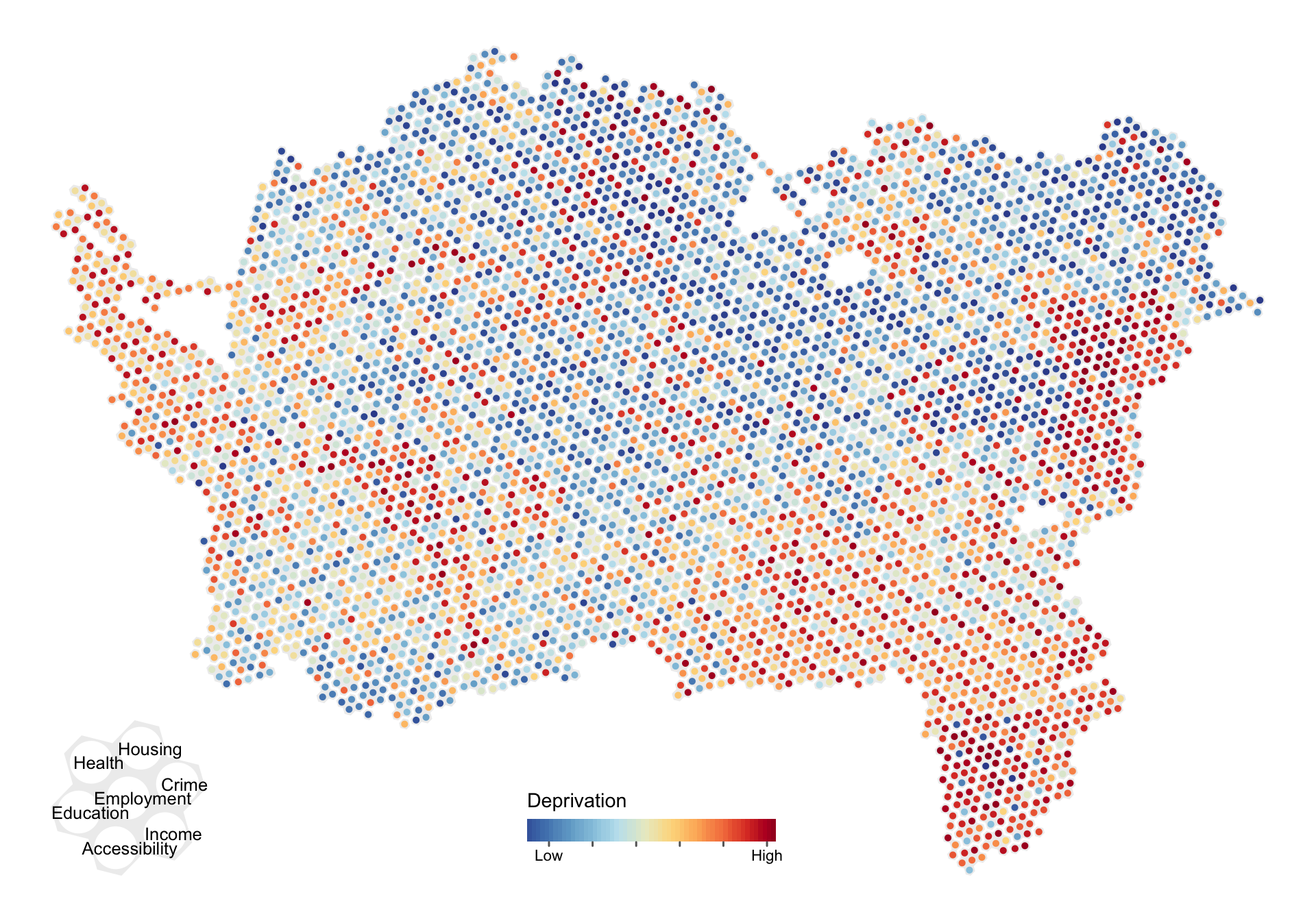

Next, one with the background ‘rosettes’ coloured by the aggregate or summary index. This is interesting because it lets you see how specific aspects of deprivation relate to the overall aggregate index.

m <- tm_shape(base) +
  tm_fill(
    fill = "Rank_IMD18", 
    fill.scale = tm_scale_continuous(
      values = "tol.sunset"),
    fill.legend = tm_legend_hide(),
    fill_alpha = 0.75)
for (i in 1:7) {
  m <- m + 
    tm_shape(layers[[i]]) + 
    tm_bubbles(
      fill = vars[i], 
      fill.scale = tm_scale_continuous(
        values = "tol.sunset"),
      fill.legend = tm_legend(
        limits = range(pull(layers[[i]], vars[i])),
        variable = "fill",
        title = "Deprivation",
        labels = c("Low", rep("", 4), "High"),
        orientation = "landscape",
        width = 15,
        position = tm_pos_in(pos.h = "center", pos.v = "bottom", just.h = 1),
        frame = FALSE,
        show = (i == 1)),
      size = 0.35,
      lwd = 0)
}
m + 
  tm_shape(legend_elements %>% slice(8)) +
  tm_fill(fill = "#eeeeee") +
  tm_shape(legend_elements %>% slice(-8)) +
  tm_dots(fill = "white", size = 2.1) + 
  tm_text(text = "dimension", size = 0.8, just = c(0.35, 0.5)) +
  tm_layout(frame = FALSE)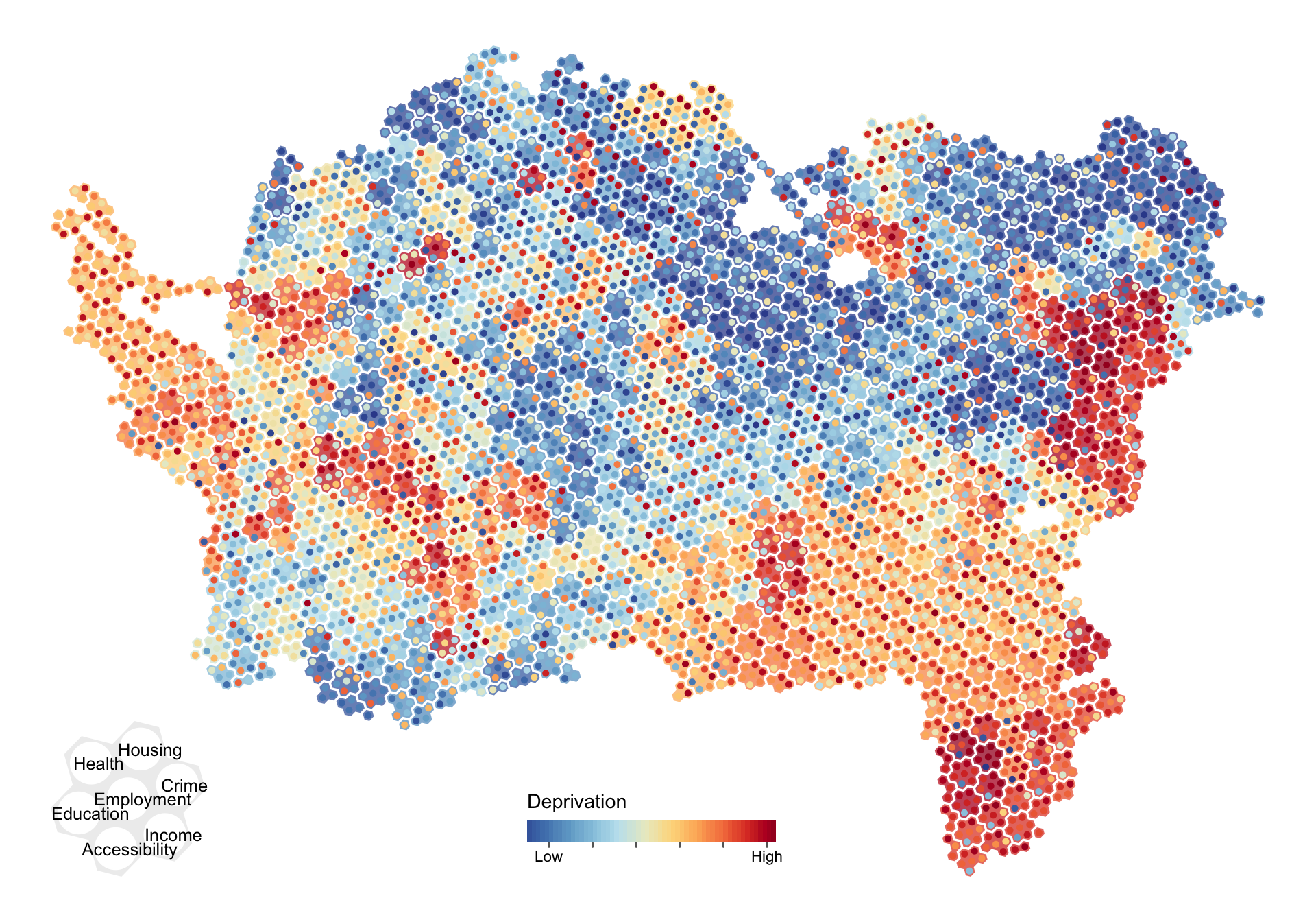

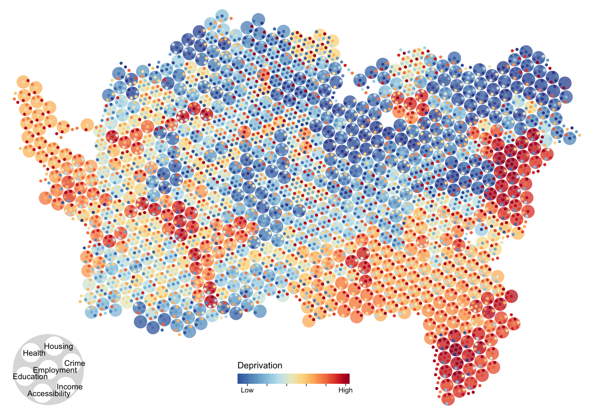
And finally, also ‘dots only’, but this time with big dots for the summary index. I think this one is the prettiest.

m <- tm_shape(layers[[1]]) +
  tm_bubbles(
    fill = "Rank_IMD18", 
    fill.scale = tm_scale_continuous(
      values = "tol.sunset"),
    fill.legend = tm_legend_hide(),
    size = 1.5,
    fill_alpha = 0.75,
    lwd = 0)
for (i in 1:7) {
  m <- m + 
    tm_shape(layers[[i]]) + 
    tm_bubbles(
      fill = vars[i], 
      fill.scale = tm_scale_continuous(
        values = "tol.sunset"),
      fill.legend = tm_legend(
        limits = range(pull(layers[[i]], vars[i])),
        variable = "fill",
        title = "Deprivation",
        labels = c("Low", rep("", 4), "High"),
        orientation = "landscape",
        width = 15,
        position = tm_pos_in(pos.h = "center", pos.v = "bottom", just.h = 1),
        frame = FALSE,
        show = (i == 1)),
      size = 0.35,
      lwd = 0)
}
m + 
  tm_shape(legend_elements %>% slice(8)) +
  tm_bubbles(fill = "#dddddd", size = 8, lwd = 0) +
  tm_shape(legend_elements %>% slice(-8)) +
  tm_dots(fill = "white", size = 2.1) + 
  tm_text(text = "dimension", size = 0.8, just = c(0.35, 0.5)) +
  tm_layout(frame = FALSE)